
Timing, profiling and compiling#
Timing#
import numpy as np
import time
rng = np.random.default_rng(3945)
A straightforward way to time code is to read the current time with time.time(). For example, consider the following matrix multiplication:
n = 10**3
A = rng.normal(size = (n,n))

t_start = time.time()
B = A@A
t_end = time.time()

print('Time taken = ', t_end-t_start)
print('GFLOPS = ', 2*n**3 / (t_end-t_start) / 1e9)
Time taken =  0.01887202262878418
GFLOPS =  105.97698187101257
As well as the time taken, this also outputs the number of floating point operations per second (in units of \(10^9\) FLOPS or GFLOPS). I’ve used the fact that for each element of the new matrix we have to do \(n\) multiplications and \(\approx n\) additions, so we expect the total number of operations to be \(2n^3\).
%%timeit -n 3 -r 10
# -n gives the number of times to run for each time measurement
# -r is the number of times to repeat the time measurement
B = A@A
21.9 ms ± 3.36 ms per loop (mean ± std. dev. of 10 runs, 3 loops each)
Question
Does the number of GFLOPS we obtain here make sense? What should it be? How does it depend on \(N\)?
Profiling#
import matplotlib.pyplot as plt
import scipy.integrate
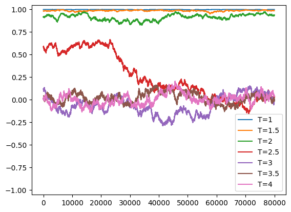
We can also look in more detail at which parts of the code take the most time. This is known as profiling. As an example, let’s take a look at the code from the homework solutions that solves the Ising model.
def run_ising(beta):

    N = 30
    Nspins = N*N
    ntrials = 10**5

    # Populate the array with random spins (+1 or -1)
    #spins = -1 + rng.integers(2, size = Nspins) * 2
    spins = np.ones(Nspins)

    M = np.zeros(ntrials)
    M[0] = np.sum(spins)/Nspins  # starting point

    # Compute the random numbers to use for accepting the jump in advance
    u = rng.uniform(size=ntrials)

    for i in range(ntrials-1):

        # Choose spin at random
        j = rng.integers(Nspins)

        # Compute energy change if this spin were to flip
        delta_E = 2*spins[j] * (spins[j-1] + spins[(j+1) % Nspins] + spins[j-N] + spins[(j+N) % Nspins])

        # Attempt flip
        if u[i] <= np.exp(-beta*delta_E):
            spins[j] = -spins[j]

        # Store magnetization
        M[i+1] = np.sum(spins)/Nspins

    # remove the first 20% (burn in)
    return M[int(ntrials/5):]
def run_ising_optimized(beta):

    N = 30
    Nspins = N*N
    ntrials = 10**5

    # Populate the array with random spins (+1 or -1)
    #spins = -1 + rng.integers(2, size = Nspins) * 2
    spins = np.ones(Nspins)

    M = np.zeros(ntrials)
    M[0] = np.sum(spins)/Nspins  # starting point

    # Compute the random numbers to use for accepting the jump in advance
    u = rng.uniform(size=ntrials)
    jvals = rng.integers(Nspins, size=ntrials)

    for i in range(ntrials-1):

        # Choose spin at random
        #j = rng.integers(Nspins)
        j = jvals[i]

        # Compute energy change if this spin were to flip
        delta_E = 2*spins[j] * (spins[j-1] + spins[(j+1) % Nspins] + spins[j-N] + spins[(j+N) % Nspins])

        # Attempt flip
        if u[i] <= np.exp(-beta*delta_E):
            spins[j] = -spins[j]
            M[i+1] = M[i] + 2*spins[j]/Nspins
        else:
            M[i+1] = M[i]

        # Store magnetization
        #M[i+1] = np.sum(spins)/Nspins

    # remove the first 20% (burn in)
    return M[int(ntrials/5):]
%%prun -q
# remove the -q above to generate output
# in class we used the profiling output to optimize--
# compare run_ising with run_ising_optimized
# with a factor of 3 speed up
T_vals = np.arange(1.0,4.05,0.1)
M_vals = np.zeros_like(T_vals)
chi_vals = np.zeros_like(T_vals)
for i, T in enumerate(T_vals):
M = run_ising(1/T)
M_vals[i] = np.mean(np.abs(M))
chi_vals[i] = np.var(M)
if (abs(np.floor(T*2)-(T*2))<1e-5):
print("T = ", T)
t = np.arange(len(M))
plt.plot(t, M, label = "T=%g" % (T,))
plt.ylim((-1.05,1.05))
plt.legend()
plt.show()
plt.clf()
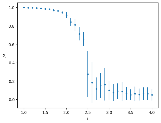
plt.errorbar(T_vals, M_vals, np.sqrt(chi_vals), fmt='.')
plt.ylabel(r'$M$')
plt.xlabel(r'$T$')
plt.show()
plt.clf()
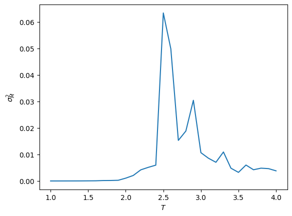
plt.plot(T_vals, chi_vals)
plt.ylabel(r'$\sigma_M^2$')
plt.xlabel(r'$T$')
plt.show()
T = 1.0
T = 1.5000000000000004
T = 2.000000000000001
T = 2.5000000000000013
T = 3.0000000000000018
T = 3.500000000000002
T = 4.000000000000003
Keeping track of memory#
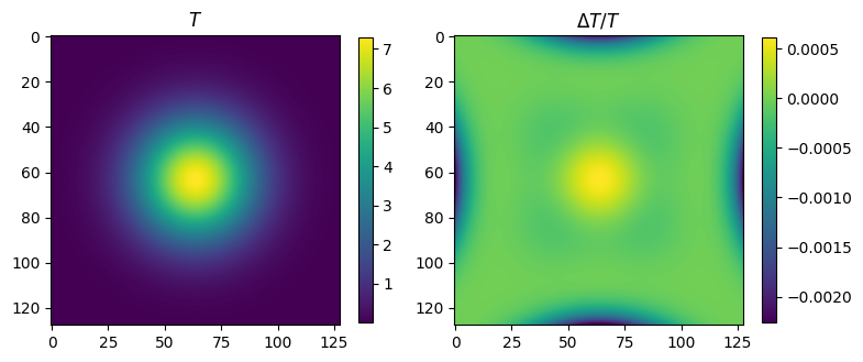
As an example, here is the code we used for 2D diffusion. We can use tracemalloc to look at the memory usage.
# MBs needed for 128x128 array of doubles
128*128*8/1e6
0.131072
import tracemalloc

tracemalloc.start()


def construct_matrices(n, alpha):
    # This is the matrix for the explicit update on the RHS
    AR = np.diag((1-alpha)*np.ones(n)) + np.diag(alpha/2*np.ones(n-1),k=1) + np.diag(alpha/2*np.ones(n-1),k=-1)

    # and for the implicit update on the LHS
    b = 1 + alpha*np.ones(n)
    a = -alpha/2*np.ones(n)
    a[0] = 0
    c = -alpha/2*np.ones(n)
    c[-1] = 0
    AL = np.row_stack((a,b,c))

    return AL, AR

def gaussian(x, y, x0, t):
    # Green's function for the diffusion equation
    dx = x-x0[0]
    dy = y-x0[1]
    return np.exp(-(dx**2 + dy**2)/(4*t)) / (4*np.pi*t)

# set up the grid and initial condition
n = 128
T = np.zeros((n,n))
x = np.linspace(0,1,n)
dx = x[1]-x[0]
xx, yy = np.meshgrid(x, x)
x0 = (0.5, 0.5)   # location of the gaussian
t0 = 0.001   # initial time
T = gaussian(xx, yy, x0, t0)

# timesteps
alpha = 2
nsteps = 80
dt = alpha * dx**2
AL, AR = construct_matrices(n, alpha)

%matplotlib
image = plt.imshow(T)
plt.title("%d: t=%lg" % (0,t0))
plt.colorbar()
plt.show()

Tnew = np.zeros_like(T)
B = np.zeros_like(T)

# We take twice as many steps here because we are doing half-timesteps
for i in range(2*nsteps):

    # Compute the right-hand side matrix row by row
    for j in range(n):
        B[j,:] = AR @ T[j,:]

    # and now solve column by column for the new T
    for j in range(n):
        Tnew[:,j] = scipy.linalg.solve_banded((1,1), AL, B[:,j])

    # take the transpose to swap directions for the next half-step
    T = Tnew.T

    if i%2 == 1:
        ti = t0 + dt*(1 + i//2)
        #plt.clf()
        #plt.imshow(T)
        #plt.title("%d: t=%lg" % (1 + i//2,ti))
        #plt.colorbar()
        #plt.show()
        #plt.pause(1e-3)

        # in class we changed the plotting to the following:
        image.set_data(T)
        plt.draw()
        plt.pause(1e-3)
        # rather than make a new plot each step, we modify the plot data

    if i%10 == 0:
        current, peak = tracemalloc.get_traced_memory()
        print("Step ", i, ": current/peak memory usage is", current / 10**6, " ", peak/10**6, "MB")

# compare the result with the analytic one
ti = t0 + dt*(1 + i//2)
delta = (T - gaussian(xx, yy, x0, ti)) / np.max(T)
print("T range = ", np.min(T), np.max(T))
print("delta range = ", np.min(delta), np.max(delta))

%matplotlib inline
plt.clf()
fig = plt.figure(figsize=(8,4))
plt.subplot(121)
plt.imshow(T)
plt.title(r'$T$')
plt.colorbar(shrink=0.7)
plt.subplot(122)
plt.imshow(delta)
plt.title(r'$\Delta T/T$')
plt.colorbar(shrink=0.7)
plt.tight_layout()
plt.show()

tracemalloc.stop()
Using matplotlib backend: <object object at 0x1057ab3b0>
Step  0 : current/peak memory usage is 1.571314   1.746036 MB
Step 10 : current/peak memory usage is 2.171768 24.627224 MB
Step 20 : current/peak memory usage is 2.211372 24.670008 MB
Step 30 : current/peak memory usage is 2.240212 24.701018 MB
Step 40 : current/peak memory usage is 2.274824 24.731646 MB
Step 50 : current/peak memory usage is 2.315045 24.781835 MB
Step 60 : current/peak memory usage is 2.325933 24.791328 MB
Step 70 : current/peak memory usage is 2.337578 24.801968 MB
Step 80 : current/peak memory usage is 2.349743 24.813838 MB
Step 90 : current/peak memory usage is 2.342981 24.822751 MB
Step 100 : current/peak memory usage is 2.355003 24.822751 MB
Step 110 : current/peak memory usage is 2.365809 24.829827 MB
Step 120 : current/peak memory usage is 2.375148 24.840051 MB
Step 130 : current/peak memory usage is 2.385793 24.850638 MB
Step 140 : current/peak memory usage is 2.378651 24.850638 MB
Step 150 : current/peak memory usage is 2.389469 24.854347 MB
T range =  7.374417235632719e-06 7.286560064543426
delta range =  -0.0022616334982004526 0.0006078416564473385
<Figure size 1280x960 with 0 Axes>
Compiling python#
Python can be slow because it is an interpreted rather than compiled language. As an example, let’s write our own implementation of matrix multiplication:
def matrix_multiply(A):
    n = np.shape(A)[0]
    B = np.zeros((n,n))
    for i in range(n):
        for j in range(n):
            for k in range(n):
                B[i,j] += A[i,k] * A[k,j]
    return B

n = 200
A = rng.normal(size = (n,n))

t_start = time.time()
B = matrix_multiply(A)
t_end = time.time()

print('Time taken = ', t_end-t_start)
print('GFLOPS = ', 2*n**3 / (t_end-t_start) / 1e9)
Time taken =  2.569782018661499
GFLOPS =  0.006226209026216856
One way to pre-compile python code is to use Cython. Let’s give it a try:
%load_ext Cython
---------------------------------------------------------------------------
ModuleNotFoundError                       Traceback (most recent call last)
Cell In[11], line 1
----> 1 get_ipython().run_line_magic('load_ext', 'Cython')

File /opt/homebrew/Caskroom/miniconda/base/lib/python3.12/site-packages/IPython/core/interactiveshell.py:2480, in InteractiveShell.run_line_magic(self, magic_name, line, _stack_depth)
   2478     kwargs['local_ns'] = self.get_local_scope(stack_depth)
   2479 with self.builtin_trap:
-> 2480     result = fn(*args, **kwargs)
   2482 # The code below prevents the output from being displayed
   2483 # when using magics with decorator @output_can_be_silenced
   2484 # when the last Python token in the expression is a ';'.
   2485 if getattr(fn, magic.MAGIC_OUTPUT_CAN_BE_SILENCED, False):

File /opt/homebrew/Caskroom/miniconda/base/lib/python3.12/site-packages/IPython/core/magics/extension.py:33, in ExtensionMagics.load_ext(self, module_str)
     31 if not module_str:
     32     raise UsageError('Missing module name.')
---> 33 res = self.shell.extension_manager.load_extension(module_str)
     35 if res == 'already loaded':
     36     print("The %s extension is already loaded. To reload it, use:" % module_str)

File /opt/homebrew/Caskroom/miniconda/base/lib/python3.12/site-packages/IPython/core/extensions.py:62, in ExtensionManager.load_extension(self, module_str)
     55 """Load an IPython extension by its module name.
     56
     57 Returns the string "already loaded" if the extension is already loaded,
     58 "no load function" if the module doesn't have a load_ipython_extension
     59 function, or None if it succeeded.
     60 """
     61 try:
---> 62     return self._load_extension(module_str)
     63 except ModuleNotFoundError:
     64     if module_str in BUILTINS_EXTS:

File /opt/homebrew/Caskroom/miniconda/base/lib/python3.12/site-packages/IPython/core/extensions.py:77, in ExtensionManager._load_extension(self, module_str)
     75 with self.shell.builtin_trap:
     76     if module_str not in sys.modules:
---> 77         mod = import_module(module_str)
     78     mod = sys.modules[module_str]
     79     if self._call_load_ipython_extension(mod):

File /opt/homebrew/Caskroom/miniconda/base/lib/python3.12/importlib/__init__.py:90, in import_module(name, package)
     88             break
     89         level += 1
---> 90 return _bootstrap._gcd_import(name[level:], package, level)

File <frozen importlib._bootstrap>:1387, in _gcd_import(name, package, level)

File <frozen importlib._bootstrap>:1360, in _find_and_load(name, import_)

File <frozen importlib._bootstrap>:1324, in _find_and_load_unlocked(name, import_)

ModuleNotFoundError: No module named 'Cython'
%%cython
# Add the flag "-a" to the line above to turn on the output

# in class we went through the modifications below
# - using cdef to declare variable types
# - using the decorators to turn off bounds checking etc.
# Basically try to turn the yellow lines in the output to white and you
# should get a significant speed up

import numpy as np

cimport cython
@cython.boundscheck(False)
@cython.cdivision(True)
@cython.wraparound(False)
@cython.initializedcheck(False)

def matrix_multiply_cython(double[:,:] A, double[:,:] B):
    cdef int i,j,k
    cdef int n = A.shape[0]
    for i in range(n):
        for j in range(n):
            for k in range(n):
                B[i,j] += A[i,k] * A[k,j]
    return B
n = 10**3
A = rng.normal(size = (n,n))
B = np.zeros_like(A)

t_start = time.time()
matrix_multiply_cython(A,B)
t_end = time.time()

print('Time taken = ', t_end-t_start)
print('GFLOPS = ', 2*n**3 / (t_end-t_start) / 1e9)
Time taken =  1.2505810260772705
GFLOPS =  1.5992566321539767
Just in time (JIT) compilation using Numba:
import numba as nb

@nb.njit(parallel = True)
def matrix_multiply(A):
    n = np.shape(A)[0]
    B = np.zeros((n,n))
    # note the use of prange in the next line for parallel loops
    for i in nb.prange(n):
        for k in range(n):
            for j in range(n):
                B[i,j] += A[i,k] * A[k,j]
    return B

n = 10**3
A = rng.normal(size = (n,n))

t_start = time.time()
B = matrix_multiply(A)
t_end = time.time()

print('Time taken = ', t_end-t_start)
print('GFLOPS = ', 2*n**3 / (t_end-t_start) / 1e9)

t_start = time.time()
B = matrix_multiply(A)
t_end = time.time()

print('Time taken = ', t_end-t_start)
print('GFLOPS = ', 2*n**3 / (t_end-t_start) / 1e9)
Time taken =  0.6430690288543701
GFLOPS =  3.110086025388297
Time taken =  0.03811812400817871
GFLOPS =  52.46847928746114
Setting parallel = True will use multiple cores with a significant speed up. It is also possible to use parallelism in Cython with OpenMP.
Other examples#
# Illustration of memory ordering
n = 10**4
A = rng.uniform(size = (n,n))
x = rng.uniform(size = n)

t_start = time.time()
for i in range(n):
    b = x * A[i,:]
t_end = time.time()

print('Time taken = ', t_end-t_start)

t_start = time.time()
for i in range(n):
    b = x * A[:,i]
t_end = time.time()

print('Time taken = ', t_end-t_start)
Time taken =  0.12569189071655273
Time taken =  0.24962282180786133
# Using built-in parallelization in scipy fft instead of numpy fft
n = 10**4
A = rng.uniform(size = (n,n))

t_start = time.time()
B = np.fft.fft(A)
t_end = time.time()
print('Time taken = ', t_end-t_start)

t_start = time.time()
B = scipy.fft.fft(A)
t_end = time.time()
print('Time taken = ', t_end-t_start)

t_start = time.time()
B = scipy.fft.fft(A, workers=8)
t_end = time.time()
print('Time taken = ', t_end-t_start)
Time taken =  1.6034882068634033
Time taken =  1.53358793258667
Time taken =  0.5826659202575684
# Demonstration of memory leak because we took a slice:
from  psutil import Process
import numpy as np

print("memory before=",Process().memory_info().rss)
arr = np.arange(0, 100_000_000)
print("memory after declaring arr=", Process().memory_info().rss)
# without the np.copy on the next line we will get a memory leak!!
small_slice = np.copy(arr[:10])
# try instead:
#small_slice = arr[:10]
del arr
print("memory after deleting arr=",Process().memory_info().rss)
memory before= 943849472
memory after declaring arr= 544079872
memory after deleting arr= 138919936
Further reading#
timeit() documentation which has details of how to call it directly from within your code or the command line.
Floating-Point Operations Per Second (FLOPS) for different architectures.
tracemalloc to profile memory usage
An interesting article on memory usage associated with NumPy slices and views