Derivatives exercises

Second order finite differences

To keep track of the error terms, write out the Taylor expansions up to the 4th order terms:

\[f(x+\Delta x) \approx f(x) + \Delta x {df\over dx} + {(\Delta x)^2\over 2}{d^2f\over dx^2} + {(\Delta x)^3\over 6}{d^3f\over dx^3} + {(\Delta x)^4\over 24}{d^4f\over dx^4}\]

\[f(x-\Delta x) \approx f(x) - \Delta x {df\over dx} + {(\Delta x)^2\over 2}{d^2f\over dx^2}-{(\Delta x)^3\over 6}{d^3f\over dx^3} + {(\Delta x)^4\over 24}{d^4f\over dx^4}\]

Then add and subtract:

\[f(x+\Delta x) + f(x-\Delta x) \approx 2f(x) + (\Delta x)^2{d^2f\over dx^2} + {(\Delta x)^4\over 12}{d^4f\over dx^4}\]

\[f(x+\Delta x) - f(x-\Delta x) \approx 2\Delta x {df\over dx} + {(\Delta x)^3\over 3}{d^3f\over dx^3}\]

Therefore

\[{d^2f\over dx^2}\approx {f(x+\Delta x) + f(x-\Delta x) -2f(x)\over (\Delta x)^2} - {(\Delta x)^2\over 12}{d^4f\over dx^4}\]

\[{df\over dx} \approx {f(x+\Delta x) - f(x-\Delta x)\over 2\Delta x} - {(\Delta x)^2\over 6}{d^3f\over dx^3}\]

For comparison, the first order derivative with the error term kept in is

\[{df\over dx} \approx {f(x+\Delta x) - f(x)\over \Delta x} - {\Delta x\over 2}{d^2f\over dx^2}\]

Optimal step size

import numpy as np
import matplotlib.pyplot as plt

def f(x):
    return np.sin(x)

dx_vals = 10**np.linspace(-13, -1, 100)

x = 1.0 # Evaluate the derivatives at this value of x

err = np.zeros_like(dx_vals)   # to store the fractional error from the 1st order difference
err2 = np.zeros_like(dx_vals)  # same for the second order

for i, dx in enumerate(dx_vals):
    dfdx1 = (f(x + dx) - f(x)) / dx
    err[i] = np.abs((dfdx1 - np.cos(x))/np.cos(x))

    dfdx2 = (f(x + dx) - f(x - dx)) / (2*dx)
    err2[i] = np.abs((dfdx2 - np.cos(x))/np.cos(x))

# Plot the results
plt.plot(dx_vals, err, label="First order")
plt.plot(dx_vals, err2, label="Second order")

plt.ylim((1e-2*min(err2), 1.0))

# and the analytic expressions
plt.plot(dx_vals, 1e-16 * f(x) / dx_vals, ":", label=r'$\epsilon f(x)/\Delta x$')
plt.plot(dx_vals, dx_vals, ":", label=r'$\Delta x$')
plt.plot(dx_vals, dx_vals**2, ":", label=r'$(\Delta x)^2$')

plt.title(r'$f(x) = \sin x, \ \ \ x=%lg$' % (x,))
plt.yscale('log')
plt.xscale('log')
plt.xlabel(r'$\Delta x$')
plt.ylabel('Fractional error in derivative')
plt.legend()
plt.show()

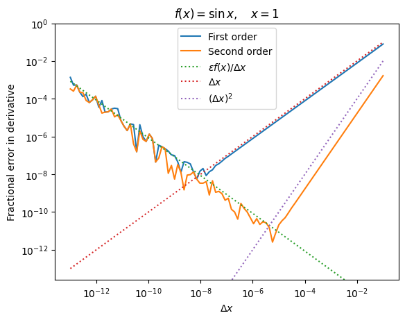
The optimal step size for the 1st order expression is \(\sim \epsilon^{1/2}\sim 10^{-8}\) and the associated error is also \(\sim \epsilon^{1/2}\).

For the second order expression, the finite difference error is \(\propto (\Delta x)^2\) rather than \(\Delta x\). Following the same argument as for the first order derivative leads to an optimal step size of order \(\epsilon^{1/3}\sim 10^{-16/3}\sim 10^{-5.3}\), and an error \(\epsilon^{2/3}\sim 10^{-10.6}\).

Notice that a higher order derivative allows us to get a better error with a larger step size.

Automatic derivatives

Inspecting the code, we can see that the operators that are implemented inside the class return a new instance of Var that is initialized with (1) the value obtained from the operation, and (2) a set of children that give the partial derivatives with respect to the variables involved in the operation.

The multiplication operator is instructive to look at. For the operation x*y, there are two variables x and y, so we need to return (1) the operation value x*y, (2) the partial derivative with respect to x, which is \(\partial(xy)/\partial x = y\), and (3) the partial derivative with respect to y, which is \(\partial(xy)/\partial y = x\). The corresponding function definition is

def __mul__(self, other):
        return Var(self.value * other.value, [(other.value, self), (self.value, other)])

For \(\exp(x)\), there is only one argument to the function so we just have to return one partial derivative \((\partial/\partial x)\exp(x) = \exp(x)\). So we can add

def exp(self):
        return Var(math.exp(self.value), [(math.exp(self.value), self)])

which we use for example as

f= x * y + x.exp()