Lorentzian fit

import numpy as np
import matplotlib.pyplot as plt

Note that for simplicity here we will set \(\sigma_i=1\) when calculating the residuals and the \(\mathbf{A}\) matrix. This means our best fit \(\chi^2\) will be \(<1\). In a real application, you would want to put these factors back in.

def lorentz(a, x, finite_difference = False):
    # Calculates the Lorentz function and the derivative with respect to the parameters
    y = a[0] / (a[1] + (x-a[2])**2)
    A =  np.zeros([len(x), len(a)])
    if finite_difference:
        eps = 1e-8
        b = a * (1+eps)
        y0 = b[0] / (a[1] + (x-a[2])**2)
        y1 = a[0] / (b[1] + (x-a[2])**2)
        y2 = a[0] / (a[1] + (x-b[2])**2)
        A[:, 0] = (y0 - y) / (b[0]-a[0])
        A[:, 1] = (y1 - y) / (b[1]-a[1])
        A[:, 2] = (y2 - y) / (b[2]-a[2])
    else:
        A[:, 0] = 1 / (a[1] + (x-a[2])**2)
        A[:, 1] = - a[0] / (a[1] + (x-a[2])**2)**2
        A[:, 2] = 2 * a[0] * (x-a[2]) / (a[1] + (x-a[2])**2)**2
    return y, A

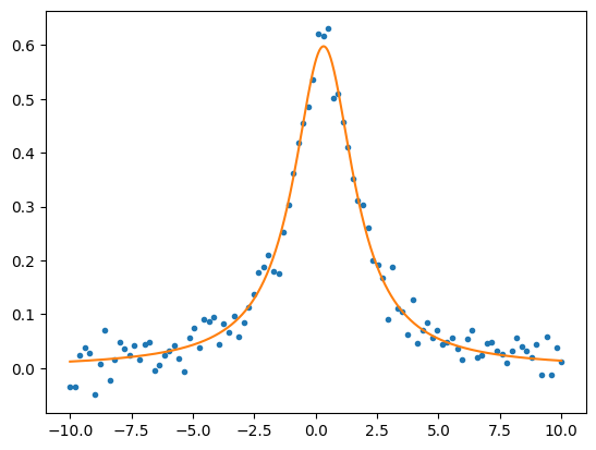
# Generate a set of "measurements" of a Lorentzian function
a0 = np.array((1.2, 2, 0.3))   # parameters of the Lorentzian
ndata = 100   # number of measurements 
x = np.linspace(-10, 10, ndata)
y, _ = lorentz(a0, x) 
y = y + 0.03 * np.random.normal(size = ndata)

# Initial guess for Newton's method
a = np.array((1,1,1))

# we have two options: analytic or numerical derivatives
finite_difference = True

# print the starting parameters and error
f, _ = lorentz(a, x, finite_difference=finite_difference)
r = y-f
last_chisq = 1e99
chisq = np.sum(r**2)
print("chisq = %g, a=(%lg, %lg, %lg)" % (chisq, a[0], a[1], a[2]))

# keep iterating while chi-squared drops by at least 1e-3
# note that this means we will also stop if chi-squared starts to increase
# which means we are not converging
while last_chisq - chisq > 1e-3:
    # calculate the update to the parameters
    f, A = lorentz(a, x, finite_difference=finite_difference)
    r = y-f
    lhs = A.T@A
    rhs = A.T@r
    da = np.linalg.inv(lhs)@rhs
    a = a + da
    # update the error
    last_chisq = chisq
    f, _ = lorentz(a, x, finite_difference=finite_difference)
    r = y-f
    chisq = np.sum(r**2)
    print("chisq = %g, a=(%lg, %lg, %lg)" % (chisq, a[0], a[1], a[2]))
    
print("a-a0 =", a-a0)

chisq = 1.65559, a=(1, 1, 1)
chisq = 0.32839, a=(1.29776, 1.84728, 0.726216)
chisq = 0.075168, a=(1.42112, 2.40337, 0.405825)
chisq = 0.0660827, a=(1.32004, 2.21729, 0.31795)
chisq = 0.0660395, a=(1.31153, 2.19465, 0.321288)
a-a0 = [0.11153324 0.19465219 0.02128819]

plt.plot(x, y, ".")

xx = np.linspace(-10, 10, 1000)
yy, _ = lorentz(a, xx)
plt.plot(xx,yy)

plt.show()

# Use the scipy least squares fitting routine to compare

import scipy.optimize

def res(a, x, y0):
    f = a[0] / (a[1] + (x-a[2])**2)
    return y-f

result = scipy.optimize.least_squares(res, (1,1,4), args=(x,y), method = 'lm')

print("Best-fit parameters are: ", result.x, " chisq = ", 2*result.cost)

plt.plot(x, y, ".")

xx = np.linspace(-10, 10, 1000)
yy, _ = lorentz(result.x, xx)
plt.plot(xx,yy)

plt.show()

Best-fit parameters are:  [1.31126399 2.19409529 0.32111827]  chisq =  0.0660395047924557

# Levenberg-Marquardt

# Note that this starting point doesn't converge for Newton!
a = np.array((1,1,4))

# we have two options: analytic or numerical derivatives
finite_difference = True

chisq1 = 1.0
chisq = 1e99
lam = 1e-3
# keep going while chisq is dropping
while chisq > 1e-6:
    # compute the update to the parameters
    f, A = lorentz(a, x, finite_difference=finite_difference)
    r = y-f
    chisq = np.sum(r**2)
    lhs = A.T@A
    lhs = lhs@(np.identity(len(a))*(1+lam))
    rhs = A.T@r
    da = np.linalg.inv(lhs)@rhs
    # calculate the chisq associated with the new parameters
    a1 = a + da
    f1, A1 = lorentz(a1, x, finite_difference=finite_difference)
    r1 = y-f1
    chisq1 = np.sum(r1**2)
    print("chisq = %lg, a=(%lg, %lg, %lg), lam = %lg" % (chisq1 ,a1[0], a1[1], a1[2], lam))
    # accept if chisq decreases; reject if it increases
    if chisq1 > chisq:
        lam = lam * 10
    else:
        lam = lam / 10
        a = a1
        # if the improvement in chisq becomes too small then exit
        if chisq-chisq1 < 1e-3:
            break
    
print("a-a0 =", a-a0)

print("Best-fit parameters are: ", a)

plt.plot(x, y, ".")

xx = np.linspace(-10, 10, 1000)
yy, _ = lorentz(a, xx)
plt.plot(xx,yy)

plt.show()

chisq = 4.23453, a=(1.11797, 2.189, 3.83747), lam = 0.001
chisq = 2.41447, a=(2.53107, 7.3536, 3.1448), lam = 0.0001
chisq = 1.10396, a=(5.93413, 21.8277, 0.471758), lam = 1e-05
chisq = 122.956, a=(-4.50563, -30.4796, 0.115764), lam = 1e-06
chisq = 123.079, a=(-4.50553, -30.4792, 0.115767), lam = 1e-05
chisq = 124.325, a=(-4.50459, -30.4745, 0.115799), lam = 0.0001
chisq = 138.926, a=(-4.49521, -30.4274, 0.116119), lam = 0.001
chisq = 193704, a=(-4.40227, -29.9618, 0.119288), lam = 0.01
chisq = 236.824, a=(-3.55657, -25.7245, 0.148127), lam = 0.1
chisq = 32.3345, a=(0.714247, -4.32601, 0.293761), lam = 1
chisq = 0.944342, a=(4.98506, 17.0725, 0.439395), lam = 10
chisq = 140.465, a=(1.14057, -1.26448, 0.308887), lam = 1
chisq = 0.80515, a=(4.28606, 13.7385, 0.415666), lam = 10
chisq = 22.1005, a=(1.37351, 0.489965, 0.318172), lam = 1
chisq = 0.685102, a=(3.75651, 11.3297, 0.39794), lam = 10
chisq = 1.17374, a=(1.50147, 1.52107, 0.323952), lam = 1
chisq = 0.582597, a=(3.3465, 9.54628, 0.384488), lam = 10
chisq = 0.27085, a=(1.56933, 2.13148, 0.3275), lam = 1
chisq = 0.0683134, a=(1.33364, 2.17595, 0.322551), lam = 0.1
chisq = 0.0660401, a=(1.31119, 2.19285, 0.321076), lam = 0.01
chisq = 0.0660395, a=(1.31124, 2.19404, 0.321114), lam = 0.001
a-a0 = [0.11124078 0.194042   0.02111426]
Best-fit parameters are:  [1.31124078 2.194042   0.32111426]