Matrices in numpy#
We’re going to be dealing with matrices quite a bit in this section, so let’s have a review of how numpy handles matrices.
import numpy as np
import matplotlib.pyplot as plt
# Matrices are 2D arrays in numpy
# A[i][j] = ith row and jth column
A = np.random.rand(12).reshape(4,3)
print(A)
print(A[1])
print(A[1][2])
print(A[1,2])
[[0.7796093  0.72652726 0.10548407]
 [0.71820389 0.96557002 0.97970296]
 [0.38199328 0.98025159 0.60079733]
 [0.89532667 0.44701858 0.48563011]]
[0.71820389 0.96557002 0.97970296]
0.9797029646146124
0.9797029646146124
# Can also use np.transpose(A)  or  A.T
A.transpose()
array([[0.7796093 , 0.71820389, 0.38199328, 0.89532667],
       [0.72652726, 0.96557002, 0.98025159, 0.44701858],
       [0.10548407, 0.97970296, 0.60079733, 0.48563011]])
# Matrix multiplication uses the @ operator
y = np.array((1,2,3))
A@y
array([2.54911601, 5.58845282, 4.14488846, 3.24625415])
# Diagonal matrix
np.diag((1,2,3,4))
array([[1, 0, 0, 0],
       [0, 2, 0, 0],
       [0, 0, 3, 0],
       [0, 0, 0, 4]])
# Inverse
np.linalg.inv((np.diag((1,2,3,4))))
array([[1.        , 0.        , 0.        , 0.        ],
       [0.        , 0.5       , 0.        , 0.        ],
       [0.        , 0.        , 0.33333333, 0.        ],
       [0.        , 0.        , 0.        , 0.25      ]])
A = np.random.rand(4).reshape(2,2)
B = np.linalg.inv(A)
B@A
array([[ 1.00000000e+00, -1.32633359e-17],
       [ 4.99998068e-17,  1.00000000e+00]])
# Determinant
print(np.linalg.det(A))
print(A[0,0]*A[1,1] - A[0,1]*A[1,0])
-0.42773786313112394
-0.42773786313112394
# should be 1 * 2 * 3 * 4 = 24
np.linalg.det(np.diag((1,2,3,4)))
23.999999999999993
Matrix decompositions#
# We need scipy.linalg for eigenvalues
import scipy.linalg

# Visualize matrices as a color map
def plot_matrices(A,titles=[]):
    n = len(A)
    if titles==[]:
        titles = [""]*n
    if n>4:
        nx = 4
    else:
        nx = n
    for j in range(int(np.floor(n/4))+1):
        plt.clf()
        plt.figure(figsize=(nx*4,4))
        jmax = 4*(j+1)
        if jmax > n:
            jmax = n
        for i,AA in enumerate(A[4*j:jmax]):
            plt.subplot(1, nx, i+1)
            plt.imshow(AA)
            plt.colorbar()
            plt.title(titles[4*j + i])
        plt.show()
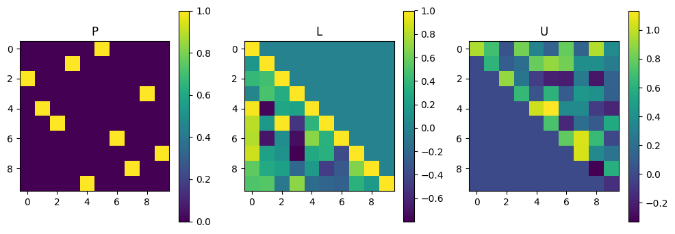
LU decomposition#
A = np.random.rand(100).reshape(10,10)
P, L, U = scipy.linalg.lu(A)
plot_matrices([P, L, U], titles=["P", "L", "U"])
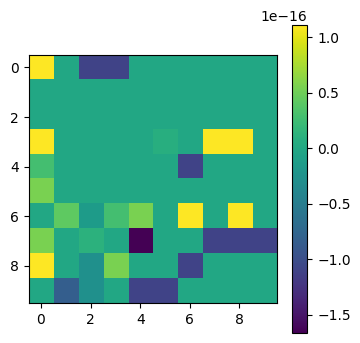
plot_matrices([P@L@U - A])
<Figure size 640x480 with 0 Axes>
<Figure size 640x480 with 0 Axes>
Eigen-decomposition#
The eigenvectors of an \(n\times n\) matrix \(\mathbf{A}\) satisfy
with eigenvalues \(\lambda_i\). Now consider the matrix \(Q\) whose columns correspond to the \(n\) eigenvectors \(\mathbf{v_i}\): you can easily show that this satisfies
where \(\mathbf{\Lambda} = \mathrm{diag}(\lambda_1, \lambda_2\dots \lambda_n)\).
Therefore
which is the eigendecomposition of the matrix.
Since \((\mathbf{A}\mathbf{B}\mathbf{C})^{-1} =\mathbf{C}^{-1}\mathbf{B}^{-1}\mathbf{A}^{-1}\), the inverse of the matrix is
where
# real symmetric matrix
n = 10
A = np.random.rand(n*n).reshape(n,n)
A = 0.5*(A + A.T)
A = A + np.diag(np.arange(n))
lam, Q = scipy.linalg.eig(A)
lam = np.real(lam)
Q = np.real(Q)

print("Eigenvalues=", lam)

print("Eigenvector check:")
for i in range(n):
    # The eigenvectors are given by the columns of Q, ie. Q[:,i]
    print(i, np.max(np.abs(A@Q[:,i]-lam[i]*Q[:,i])))
Eigenvalues= [11.28458032  0.0868573   9.12730965  7.7116523   1.36434437  6.28607079
  5.71343268  2.4509571   3.64049758  3.93367003]
Eigenvector check:
0 5.329070518200751e-15
1 2.1649348980190553e-15
2 8.548717289613705e-15
3 4.107825191113079e-15
4 3.073929999430902e-15
5 2.9976021664879227e-15
6 2.6645352591003757e-15
7 2.5673907444456745e-15
8 8.881784197001252e-16
9 1.4849232954361469e-15
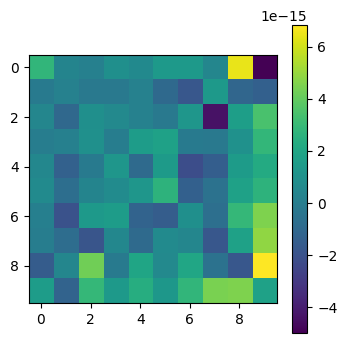
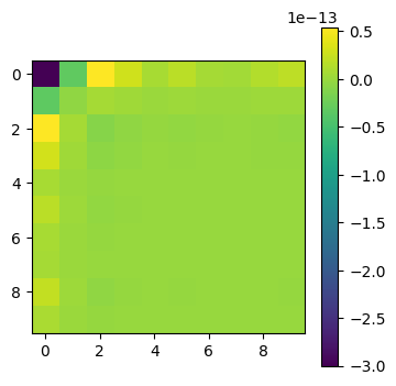
# Check eigendecomposition
plot_matrices([Q@np.diag(lam)@np.linalg.inv(Q) - A])
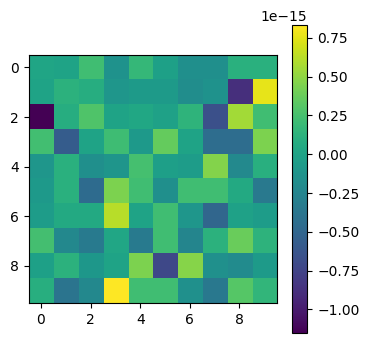
# and the inverse
plot_matrices([Q@np.diag(1/lam)@np.linalg.inv(Q) - np.linalg.inv(A)])
<Figure size 640x480 with 0 Axes>
<Figure size 640x480 with 0 Axes>
plot_matrices([np.linalg.inv(Q) - Q.T])
<Figure size 640x480 with 0 Axes>
Singular value decomposition (SVD)#
The singular value decomposition (SVD) of a \(m\times n\) matrix \(\mathbf{A}\) is
where
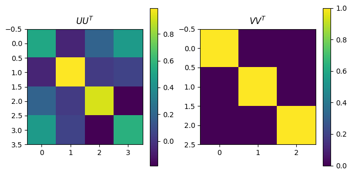
\(\mathbf{U}\) is an \(m\times n\) matrix with orthonormal columns
\(\mathbf{S}\) is an \(n\times n\) diagonal matrix whose diagonal elements are the singular values of the matrix \(s_i\)
\(\mathbf{V}\) is an \(n\times n\) orthogonal matrix (\(V^TV = VV^T = 1\))
If we have a square matrix (\(m=n\)), we can write the inverse as
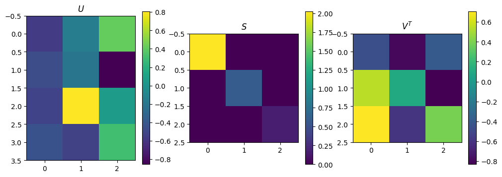
m=4; n=3
A = np.random.rand(m*n).reshape(m,n)
U, Sdiag, VT = np.linalg.svd(A, full_matrices=False)
print("Singular values are: ", Sdiag)
S = np.diag(Sdiag)
plot_matrices([U, S, VT], titles=[r"$U$", r"$S$", r"$V^T$"])
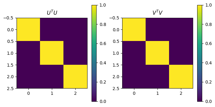
# U and V should be orthogonal
plot_matrices([U.transpose()@U,VT@VT.transpose()], titles=[r"$U^TU$",r"$V^TV$"])
plot_matrices([U@U.transpose(),VT.transpose()@VT], titles=[r"$UU^T$",r"$VV^T$"])
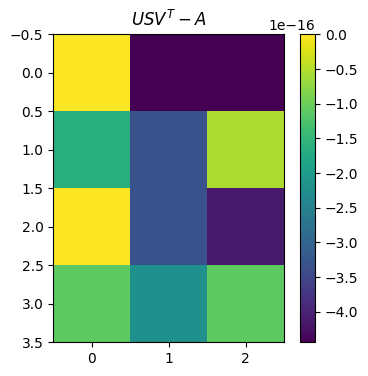
# Check the reconstructed matrix
plot_matrices([U@S@VT - A], titles=[r"$USV^T - A$"])
Singular values are: [2.0219815 0.58925587 0.17027338]
<Figure size 640x480 with 0 Axes>
<Figure size 640x480 with 0 Axes>
<Figure size 640x480 with 0 Axes>
<Figure size 640x480 with 0 Axes>