Homework 6

Due on Tuesday Nov 21 by midnight.

1. Pseudo-Hamiltonian for the simple harmonic oscillator   [Solution]

This question builds on the in-class exercise that we did on symplectic integrators.

(a) Use the Jacobian for the leapfrog method to show that the pseudo-Hamiltonian

\[\tilde{H}(h) = {1\over 2}x^2 + {1\over 2} v^2 {1\over 1-h^2/4}\]

is conserved when using the leapfrog method. (As in the in-class exercise, I’ve set the mass, spring constant, and oscillator frequency to 1 for simplicity here.)

(b) Implement the leapfrog method for the simple harmonic oscillator numerically. Check that your integrations do indeed conserve \(\tilde{H}\).

(c) Use your code from part (b) to calculate the scaling of the energy error with the number of steps per oscillation cycle for integrations of (1) a whole oscillation and (2) half an oscillation. Discuss whether the scalings you find agree with the analytic results for the leapfrog method.

2. Eigenvalue problem for the wave on a string   [Solution]

(a) Show that the difference equations for a wave on a string can be written in the form

\[\mathbf{A}\cdot\mathbf{f} = \omega^2 \mathbf{b}\cdot\mathbf{f},\]

where \(\mathbf{A}\) is a tridiagonal matrix, and \(\mathbf{b}\) is a diagonal matrix.

(The easiest way to do this is to exclude the boundary points where \(f=0\) from your grid, so that your grid involves only the interior points. Then your matrices will take a simple form.)

(b) Use scipy.linalg.eigh to solve for the eigenvalues and eigenvectors.

Plot the first 8 eigenfunctions \(f(x)\) and compare the frequencies with our results from the shooting method. Do this for both a constant density string and a string with density \(\propto 1+10x^2\).

3. Leapfrogging an electromagnetic wave   [Solution]

You have probably seen the reflection and transmission coefficients for electromagnetic waves when they propagate across a boundary:

\[r = {n_2-n_1\over n_2+n_1}, \hspace{1cm} t = {2n_1\over n_2+n_1}.\]

Let’s check these by directly integrating the wave equation!

Maxwell’s equations for an electromagnetic wave propagating in the \(x\)-direction in a material with refractive index \(n\) can be written

\[{\partial B\over \partial t} = -{\partial E\over \partial x}, \hspace{1.5cm}{\partial E\over \partial t} = -{1\over n(x)^2}{\partial B\over \partial x}\]

where \(E\) and \(B\) are the electric and magnetic fields and we have set the speed of light \(c=1\) for simplicity. Writing down a second-order finite difference approximation for both the space and time derivatives gives the update scheme

\[B^{n+1}_i = B^{n-1}_i - {\Delta t\over \Delta x} \left(E^n_{i+1}-E^n_{i-1}\right)\]

\[E^{n+1}_i = E^{n-1}_i - {\Delta t\over \Delta x} \left(B^n_{i+1}-B^n_{i-1}\right){1\over n_i^2}.\]

Here subscript \(i\) labels the grid cell and superscript \(n\) the time step. To find the values at time \(n+1\) requires storing both values from the previous two timesteps, \(n\) and \(n-1\). This is another example of a leapfrog method.

(a) First code up this algorithm and set the refractive index \(n=1\) across the grid. Start with a Gaussian profile centered on your grid. Choose \(E\) and \(B\) to have the same profile, but try giving them either the same sign or opposite signs. What difference does that make? Does the Gaussian propagate without changing shape?

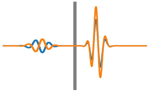
(b) Now set \(n=n_1\) on the left half of your grid and \(n=n_2\) on the right. Start a pulse in the left half moving towards the right (Hint: for \(n\) not equal to 1 you will need to set \(nE\) and \(B\) to have the same profile to get the wavepacket moving in one direction). Do you see the expected behaviour of the wave amplitude when the pulse encounters the change in \(n\) at the middle of the grid?

Some hints:

• The simplest spatial boundary conditions to use are periodic, so for example if you have \(N\) grid cells from \(i=1\) to \(N\), then you take \(E_{N+1}=E_1\) and \(E_0 = E_N\) when updating the points at the edge of the grid (and same for \(B\)). This let’s you use np.roll to do the update.

• For the first time step, you can take a first order step to get the integration going:

\[B^1_i = B^0_i - {\Delta t\over \Delta x} \left(E^0_{i+1}-E^0_{i-1}\right)\]

\[E^1_i = E^0_i - {\Delta t\over \Delta x} \left(B^0_{i+1}-B^0_{i-1}\right){1\over n_i^2}.\]

• For the method to be stable you will need to choose \(\alpha = \Delta t/\Delta x<1\) (try a larger value and you will see what happens!)