
Linear Congruential Generators#
These widely-used generators are of the form
Notes:
The starting value of \(X\) is the seed. If the sequence ever produces the seed again at a later iteration, it will start over with the same sequence of numbers. How long this takes is the period of the generator.
The modulus \(m\) sets the maximum period of the random number sequence (although the period can be much smaller for bad choices of \(a\) and \(c\)).
To return a floating point number between 0 and 1, we can divide by \(m\).
A list of different choices of parameters is given on the Wikipedia page for linear congruential generators – we explore some of these below and compare with the build in numpy generator. (Note that you should always use a well-tested generator like the numpy one rather than coding your own, the tests below should show you why!)
import numpy as np
import matplotlib.pyplot as plt
# This is the implementation of an LCG from Wikipedia
# https://en.wikipedia.org/wiki/Linear_congruential_generator
# (simplified by removing type info)

def lcg(modulus, a, c, seed):
    """Linear congruential generator."""
    while True:
        seed = (a * seed + c) % modulus
        yield seed
# Make some plots to compare different choices of LCG parameters
params = []
# the parameters are: m, a, c, seed, name
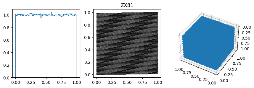
params.append([2**16+1, 75, 74, 33, "ZX81"])
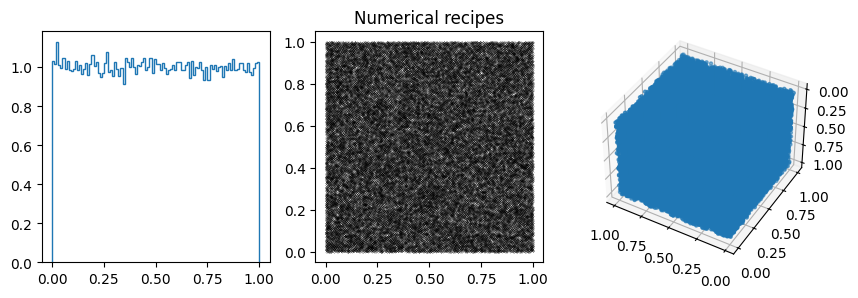
params.append([2**32, 1664525, 1013904223, 33, "Numerical recipes"])
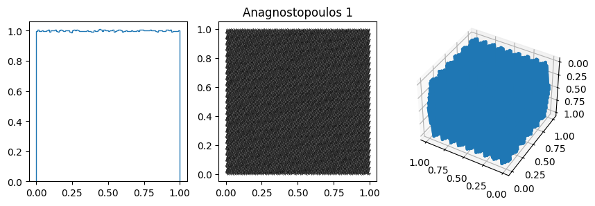
params.append([2**17, 1277, 0.0, 13337, "Anagnostopoulos 1"])
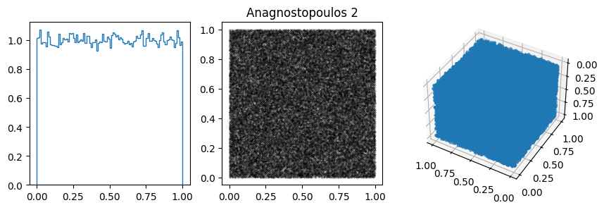
params.append([2**31-1, 7**5, 0.0, 323412, "Anagnostopoulos 2"])
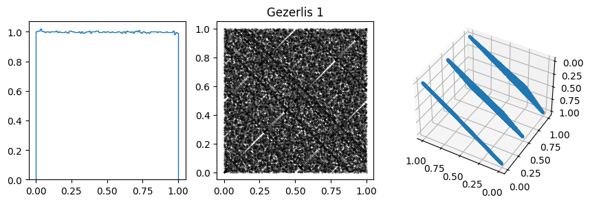
params.append([2**32, 2**18 + 1, 7, 33, "Gezerlis 1"])
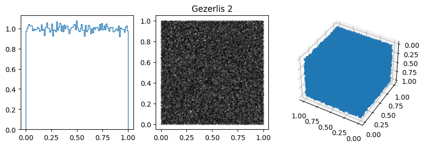
params.append([2**32, 1812433253, 7, 33, "Gezerlis 2"])
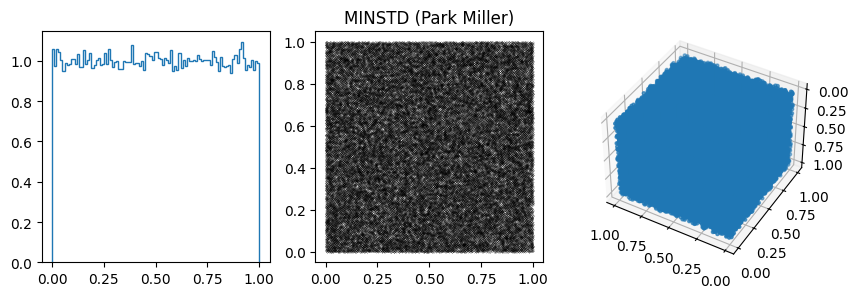
params.append([2**31-1, 7**5, 0, 33, "MINSTD (Park Miller)"])
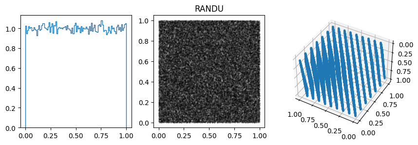
params.append([2**31, 65539, 0, 33, 'RANDU'])
params.append([-1, -1, -1, 56, "Numpy"])
for m, a, c, seed, name in params:
if m == -1:
samples = np.random.default_rng(seed).uniform(size = 10**5)
else:
samples = np.fromiter(lcg(m, a, c, seed), float, count = 10**5)
samples = samples/m
plt.clf()
fig = plt.figure(figsize=(10,3))
# 1D distribution
ax1 = fig.add_subplot(131)
ax1.hist(samples, density=True, bins=100, histtype = 'step')
# 2D x_i against x_{i+1}
ax2 = fig.add_subplot(132)
ax2.plot(samples[1:], samples[:-1], 'k.', ms=0.2)
plt.title(name)
# 3D x_i, x_{i+1} and x_{i+2}
ax3 = fig.add_subplot(133, projection='3d')
# zoom in on part of the data
#cutoff = 0.05
#samples = samples[np.where(samples<cutoff)]
#ax3.set_xlim(0,cutoff)
#ax3.set_ylim(0,cutoff)
#ax3.set_zlim(0,cutoff)
ax3.scatter(samples[:-2], samples[1:-1], samples[2:], marker='.')
ax3.view_init(-140, 60)
plt.show()
<Figure size 640x480 with 0 Axes>
<Figure size 640x480 with 0 Axes>
<Figure size 640x480 with 0 Axes>
<Figure size 640x480 with 0 Axes>
<Figure size 640x480 with 0 Axes>
<Figure size 640x480 with 0 Axes>
<Figure size 640x480 with 0 Axes>
<Figure size 640x480 with 0 Axes>
<Figure size 640x480 with 0 Axes>

Notes:
You can often spot the bad generators from the bin-to-bin variations of the 1D distribution. (E.g. ZX81, Anagnostopoulos 1 and Gezerlis 1 all have smaller than expected variance.) One other thing we could look at is how the bin-to-bin variations scale with the number of samples (expect the standard deviation from a uniform distribution to go down as \(1/\sqrt{N}\).
In other cases, the 1D distribution looks acceptable, but you can see correlations in the 2d plot, ie. successive samples are correlated. In others, e.g. RANDU, these emerge in the 3D plots.
These generators all have the property that when used to make a \(n\)-d plot, the points do not fill up the whole space, but instead lie on \((n-1)\)d hyperplanes (so 2d planes in the 3d plot or lines in the 2d plot). There are at most about \((n! m)^{1/n}\) planes, which is not that large, e.g. \(m=2^{31}\) then for \(n=3\) we get \((6m)^{1/3}\sim 2300\).
A related issue with these generators is that often the least significant bits are much less random then the most significant bits. E.g. change the 2D plots to log-log and look at the behavior of small numbers, for example in MINSTD.
Further reading
More on RANDU, which was used a lot in the 1960s and 1970s, but as we saw above is not a good generator, with significant correlations.
Remarks on choosing and implementing random number generators
Documentation for NumPy’s random sampling routines can be found at
numpy.randomincluding the PCG64 generator which is the default generator in numpy. Note that is has a period of \(2^{128}\) (\(\sim 10^{38}\)), much larger than the examples above!Having a high quality random number generator is particularly important for cryptography. A starting point is the wikipedia article on Cryptographically secure pseudorandom number generator.
NIST provides software for testing random number sequences: Random Bit Generation at NIST