Boundary value problems

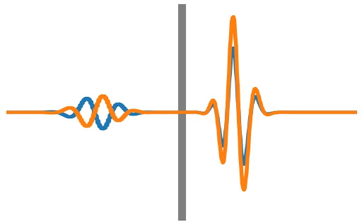
Another class of ODE problems are boundary-value problems in which we need to satisfy boundary conditions at different locations. The example we’ll use is a wave on a string, which is governed by the equation

\[\rho(x) {\partial^2 \xi\over \partial t^2} - T{\partial^2 \xi\over\partial x^2} = 0,\]

where \(\xi\) is the vertical displacement (assumed small), \(T\) is the tension (assumed constant), and \(\rho(x)\) is the mass per unit length, which here we take to depend on the coordinate \(x\) along the string. If the string is fixed at both ends, we have a boundary value problem in which \(\xi=0\) at both \(x=0\) and \(x=L\).

For a normal mode of the string \(\xi\propto e^{i\omega t}\), the governing equation reduces to the ODE

\[{d^2\xi\over d x^2} = -{\omega^2 \rho(x)\over T} \xi.\]

There are two different techniques we can use to solve this: shooting or relaxation.

Shooting method

In the shooting method, the idea is to start on one side, integrate across to the other boundary and then check whether the boundary condition is satisfied there. If not, we need to adjust either the conditions at the starting point or a parameter in the equations (here we’ll be adjusting the mode frequency \(\omega\)) and try again. By iterating, you can converge on the correct value of the parameter which gives both boundary conditions satisfied.

Since we have a second order differential equation, the first thing to do is to rewrite the equation as two first order ODEs,

\[{df\over dx} = g\]

\[{dg\over dx} = -{\omega^2 \rho(x)\over T} f.\]

At the left boundary, \(x=0\), we have \(f=0\) as one of our boundary conditions. We also need a starting value of \(g\) and we need to choose a value for \(\omega\). This particular problem is linear, so the solution \(f\) can be rescaled and still satisfy the equations. This means that the choice of \(g\) just acts as an overall scaling for the solution: we can set \(g=1\) for example (or any other value). The parameter that we need to tune to be able to match the boundary condition at \(x=L\) (we need \(f=0\) at \(x=L\)) is the mode frequency \(\omega\). This is the eigenvalue of the problem: only for particular choices of \(\omega\) will we find solutions that satisfy both of our boundary conditions.

So the procedure is:

1. Choose an initial guess for \(\omega\) and start at \(x=0\) with \(f=0\) and \(g=1\).

2. Integrate the coupled ODEs across to \(x=L\).

3. Check whether \(f=0\) at \(x=L\) and if not, adjust \(\omega\) and try again.

4. Repeat until the boundary condition at \(x=L\) is satisfied to some target accuracy or until the value of \(\omega\) stops changing to some target accuracy.

Exercise: waves on a string

Implement the shooting method to find the first 6 eigenmodes and eigenfrequencies of the string. Start with a constant density string and check that you get the expected solution. Then try a density \(\rho = 1 + 10 (x/L)^2\), so that the string is much heavier at one end compared to the other.

You can use scipy.integrate.solve_ivp to do the integration, and a root finder such as scipy.optimize.brentq to find the value of \(\omega\) that zeros the right hand boundary condition.

For example:

def do_integration(omega):
    # Returns f(x=L) given the trial frequency omega 
    result = < do integration for this value of omega >
    return < value of f at x=L >

# Search for the root between frequencies om1 and om2
omega = scipy.optimize.brentq(do_integration, om1, om2)

[Solution]

Relaxation method

Relaxation methods take a different approach: guess the solution \(f(x)\) and iteratively refine the solution until it satisfies the differential equation.

For this method, we can work with the second order equation

\[{d^2 f\over d x^2} = -{\omega^2 \rho(x)\over T} f.\]

Let’s assume that we know the frequency \(\omega\) and want to solve for the eigenfunction \(f(x)\). Set \(T=1\) for simplicity and finite-difference the equation on a grid in \(x\):

\[{f_{i+1}-2f_i+f_{i-1}\over (\Delta x)^2} = - \omega^2\rho_i f_i,\]

where \(\rho_i\) is the density at \(x=x_i\). Now write this with a zero on the right hand side:

(10)\[G_i \equiv f_{i+1} - \left[2 - (\Delta x)^2\omega^2\rho_i)\right] f_i+f_{i-1} = 0.\]

We need to find the \(N\) values of \(f_i\) that zero the \(N\) functions \(G_i\) (where \(N\) is the number of grid points). We just have to be careful at the boundaries: since we need \(f\) to vanish at the boundaries, the appropriate values of \(G\) there are

\[G_1 = f_1 = 0 \hspace{1cm} G_N = f_N=0,\]

and \(G_i\) is given by (10) for \(i=2\) to \(N-1\).

We can find the root using Newton’s method. Given a current guess \(f^n_i\) and the corresponding \(G^n_i\)’s (\(n\) labels the iteration), we make a first order Taylor expansion and set it to zero to estimate the values \(f^{n+1}_i\) that will zero the \(G_i\)’s:

\[G^{n+1}_i = G^n_i + {\partial G^n_i\over \partial f_j}(f_j^{n+1}-f_j^n) = 0.\]

Defining the Jacobian matrix \(J_{ij} = \partial G_i/\partial f_j\), the new values \(f^{n+1}_j\) are given by

\[G^{n+1}_i = G^n_i + J_{ij}(f_j^{n+1}-f_j^n) = 0\]

or

\[f_j^{n+1} = f_j^n - (J^{-1})_{ji} G^n_i.\]

If the initial guess is good enough, this should converge on the correct solution.

Exercise: waves on a string with relaxation

Take one of the eigenfrequencies that you found in the previous exercise, and use the relaxation method to find the eigenfunction corresponding to that frequency.

Do you get good agreement with the eigenfunctions from the shooting method? How many grid points do you need to get a good solution? Does the starting guess make a difference?

You can calculate the Jacobian either by implementing the analytic Jacobian (you will see that the matrix is of tridiagonal form so fairly easy to calculate) or using finite differences.

[Solution]