Week 7 Solutions - PHYS 633 Astrophysical Dynamics

Reading questions¶

Chaos is a word used to describe systems whose outcomes are extremely sensitive to initial conditions. Despite this, the system remains deterministic, meaning the future state of a system is completely determined by its current state and the laws governing it (so nothing random!). However any small deviations from initial conditions can lead to exponentially different evolutions. With regards to the Solar System, the text explicitly states: “An object in the solar system can be said to exhibit chaotic motion if its final dynamical state is sensitively dependent on its initial state.”
a) Recall from Chapter 3 of Murray and Dermott for the case of a planar, circular restricted three-body problem, there exists a constant of motion defined by

C_J=n^2(x^2+y^2)+2\left(\frac{\mu_1}{r_1}+\frac{\mu_2}{r_2}\right)-\dot{x}^2-\dot{y}^2.

Because of the existence of the Jacobi constant, which can be fixed, only 3 variables need to be determined, and the 4th can be extracted from the above equation. That is, any permutaion of $C_J$ with three of $(x,y,\dot{x}, \dot{y})$ . This reduction in dimensionality means that the path of the particle in phase space is restricted to live on a surface (Think of how we defined the equation for a surface in linear algebra. For the linear case, it is given by $ax+by+cz=d$ where (a,b,c,d) are constants. We have a similar situation here except it’s a 3D surface embedded in 4D space). Now this reduction allows us to define the Pointcaré surface of section. This is done by choosing a Jacobi constant to set up a surface, and plotting points only when they cross this surface. So we have gone from $R^4 (\text{phase space path of particle}) \rightarrow R^3 (\text{Jacobi surface}) \rightarrow R^2 (\text{Poicaré surface of section, or points})$ . This is useful in illustrating the regular and chaotic regions of an orbit.

b) Mathematically, its the set of all positions and velocities that a test particle is allowed to have for a fixed value of the Jacobi constant in the circular restricted three-body problem. Because the Jacobi constant combines kinetic energy and an effective potential in the rotating frame, the Jacobi surface acts like an energy constraint: the particle’s motion is confined to this surface and cannot access regions of phase space that would violate that energy balance. It fixes where the particle can move and how fast it can move.

The islands are a characteristic of resonant motion. In the case where we have a mean motion resonance of $p+q:p$ , we would have $q$ islands. The center of each island would be a stable periodic orbit in exact resonance, while the surrounding closed curves correspond to quasi-periodic librations about that periodic configuration. Physically, the islands represent regions of stable resonant trapping where conjunctions occur in a repeating geometric pattern and the motion is dynamically protected from chaotic diffusion. Its interesting to note that points appear successively at one different island every time, they don’t ‘trace out’ one island, then move to the next.
As alluded to above, placing the particle at the staring condition for the island that straddles $\dot{x}=0$ yields a trajectory that would appear as a succession of three points, one at the centre of each island in turn. This is because the centre of each island corresponds to a starting condition that places the test particle at the middle of the resonance. By moving the starting location further away from the centre, the islands would get larger, corresponding to larger variations in $e$ and $a$ .
For two orbits separated in phase space by a distance $d_0$ at time $t_0$ . Let $d$ be their separation at time $t$ . The orbit is chaotic if $d$ is approximately related to $d_0$ by the \textbf{Lyapounov exponent} $\gamma$ in

d=d_0\text{ exp}\gamma (t-t_0).

The maximum Lyapunov characteristic exponent (LCE) measures the rate at which nearby trajectories in phase space diverge. A positive LCE indicates chaos, meaning small differences in initial conditions grow exponentially over time, while a zero or negative LCE corresponds to regular, stable motion. It provides a quantitative measure of sensitive dependence on initial conditions.

The problem with the perturbation expansion is that although the expansion is done in powers of small parameters, the existence of resonances between the planets will introduce small divisors into the expansion terms. Such small divisors can make high order ter ms in the power series unexpectedly large and destroy the convergence of the series.
One of the many examples: In 2016, Japanese physicists published a paper titles ‘The motion of Pluto over the age of the solar system’ where they carried out the numerical integration of Pluto over the age of the solar system (5.7 billion years towards the past and 5.5 billion years towards the future). They found that the time evolution of Keplerian elements of a nearby trajectory of Pluto at first grow linearly with the time and then start to increase exponentially. These exponential divergences stop at about 420 Myr and saturate. The exponential divergences are suppressed by three resonances that Pluto has.
The general consensus it that the Solar System exhibits chaotic behavior, particularly in the inner planets, with Lyapunov timescales of a few million years (Laskar 1989, 1990; Sussman & Wisdom 1992). The outer planets and Pluto also show signs of chaos, though on slightly longer timescales, and the chaotic behavior of Pluto appears largely independent of the giant planets.
At the same time, the Solar System has survived for billions of years, suggesting that the chaotic regions are narrow and the system is globally stable, at least over the timescales explored in the simulations. In other words, the Solar System is probabilistically stable: most configurations remain regular, but precise long-term predictions are limited by chaos.

Numerical exercise: 3-body simulations & Chaos & Resonance¶

import matplotlib.pyplot as plt
import rebound
import time
import numpy as np
plt.close()


def to_rot_frame(zeta, eta, l):
    x = np.cos(l)*zeta + np.sin(l)*eta
    y = -np.sin(l)*zeta + np.cos(l)*eta
    return np.array([x, y])


plt.rcParams['xtick.direction'] = 'in'
plt.rcParams['ytick.direction'] = 'in'
plt.rcParams['xtick.top'] = True
plt.rcParams['ytick.right'] = True

Orbits are sensitive to initial conditions. Now place 2 particles with the same semi-major axis ( $a_0 = 0.8$ ), eccentricity ( $e_0 = 0.4$ ) and longitude of pericentre ( $\bar{\omega} = 295^\circ$ ) but with slightly different initial mean longitudes ( $\theta = 293^\circ$ and $\theta = 293.5^\circ$ ). Run the simulation for 1 period of Jupiter’s orbit. Can you see the deviation?

mu2 = 1e-3
mu1 = 1 - mu2

# setup simulations
sim = rebound.Simulation()
sim.add(m = mu1, hash = "star")
sim.add(m = mu2, a = 1, hash = "jupiter")
sim.add(m=0, a=0.8, e=0.4, 
        pomega = 295/180*np.pi, l = 293/180*np.pi,
        hash = "test_1")
sim.add(m=0, a=0.8, e=0.4, 
        pomega = 295/180*np.pi, l = 293.5/180*np.pi,
        hash = "test_2")

sim.move_to_com()
p_orb    = 2*np.pi
num_orb  = 1
Noutputs = 360*num_orb
times    = np.linspace(0, num_orb*2*np.pi, Noutputs)


tp_x = np.zeros((2, Noutputs))
tp_y = np.zeros((2, Noutputs))

ang_p = np.zeros(Noutputs)

for i, t in enumerate(times):
    sim.integrate(t)
    for k in range(2):
        tp_x[k, i] = sim.particles[k+2].x
        tp_y[k, i] = sim.particles[k+2].y
    orb_p = sim.particles["jupiter"].orbit(primary = sim.particles["star"])
    ang_p[i] = orb_p.theta


tp_x[0], tp_y[0] = to_rot_frame(tp_x[0], tp_y[0], ang_p)
tp_x[1], tp_y[1] = to_rot_frame(tp_x[1], tp_y[1], ang_p)


fig, ax = plt.subplots(1, 1)

ax.plot(tp_x[0], tp_y[0], label = r"$\theta = 293^\circ$")
ax.plot(tp_x[1], tp_y[1], label = r"$\theta = 293.5^\circ$")
ax.scatter(-mu2, 0, color = "orange", s=30)
ax.scatter(mu1, 0, color = "black", s=10, zorder= 2)

ax.text(-mu2, 0.2, "Sun", color = "orange")
ax.text(mu1 -0.3, -0.5, "Jupiter",  color = "black")

ax.set_aspect('equal', 'box')
ax.set_xlim(-3, 3)
ax.set_ylim(-3, 3)
plt.legend()
plt.show()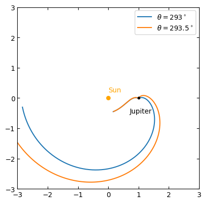

mu2 = 1e-3
mu1 = 1 - mu2
C_j = 3.07


# location 1: stable
a01 = 0.6944
e01 = 0.2065
# location 2: chaotic
a02 = 0.6984
e02 = 0.1967
# small deviation for the pair of particles at each loc
devi = 0.00005

a01d, e01d = a01 + devi, e01 + devi
a02d, e02d = a02 + devi, e02 + devi

# or get location a,e with Murray function 9.5
def get_ae_from_x0(x0, devi = 0, Cj = C_j):
    x0  += devi
    y0  = 0 + devi
    print("for the value of x0:", x0)
    r10     = x0 + mu2
    r20     = mu1 - x0
    vx0_rot = 0
    vy0_rot = np.sqrt(x0**2 + y0**2 + 2*(mu1/r10 + mu2/r20) -vx0_rot**2 - Cj)

    vx0     = vx0_rot - y0 
    vy0     = vy0_rot + x0

    V2      = vx0_rot**2 + (vy0_rot + x0 + mu2)**2
    h2      = ((x0 + mu2)*(vy0_rot + x0 + mu2))**2

    a00 = 1/(2/r10 - V2/mu1)
    e00 = np.sqrt(1- h2/(a00*mu1))
    print("you get:", a00, e00)
    return a00, e00, vx0, vy0


x0_pack = [0.55, 0.55001, 0.56, 0.56001]

a01,  e01,  vx01,  vy01  = get_ae_from_x0(x0_pack[0])
a01d, e01d, vx01d, vy01d = get_ae_from_x0(x0_pack[1])
a02,  e02,  vx02,  vy02  = get_ae_from_x0(x0_pack[2])
a02d, e02d, vx02d, vy02d = get_ae_from_x0(x0_pack[3])


# setup simulations
sim = rebound.Simulation()
sim.add(m = mu1, hash = "star")
sim.add(m = mu2, a = 1, hash = "jupiter")
sim.move_to_com()

# sim.add(m=0, a=a01, e=e01, hash = "loc1")
# sim.add(m=0, a=a01d, e=e01d, hash = "loc1_d")
# sim.add(m=0, a=a02, e=e02, hash = "loc2")
# sim.add(m=0, a=a02d, e=e02d, hash = "loc2_d")

sim.add(m=0, x=x0_pack[0], y=0, vx=vx01, vy=vy01, hash = "loc1")
sim.add(m=0, x=x0_pack[1], y=0, vx=vx01d, vy=vy01d, hash = "loc1_d")
sim.add(m=0, x=x0_pack[2], y=0, vx=vx02, vy=vy02, hash = "loc2")
sim.add(m=0, x=x0_pack[3], y=0, vx=vx02d, vy=vy02d, hash = "loc2_d")

p_orb    = 2*np.pi
num_orb  = 300
Noutputs = 360*num_orb
times    = np.linspace(0, num_orb*2*np.pi, Noutputs)


tp_a = np.zeros((4, Noutputs))
tp_e = np.zeros((4, Noutputs))
tp_x = np.zeros((4, Noutputs))
tp_y = np.zeros((4, Noutputs))

tp_vx = np.zeros((4, Noutputs))
tp_vy = np.zeros((4, Noutputs))

ang_p = np.zeros(Noutputs)

for i, t in enumerate(times):
    sim.integrate(t, exact_finish_time=1)

    for k in range(4):
        tp_a[k, i] = sim.orbits()[k+1].a
        tp_e[k, i] = sim.orbits()[k+1].e
        tp_x[k, i] = sim.particles[k+2].x
        tp_y[k, i] = sim.particles[k+2].y
        tp_vx[k, i] = sim.particles[k+2].vx
        tp_vy[k, i] = sim.particles[k+2].vy

    orb_p = sim.particles["jupiter"].orbit(primary = sim.particles["star"])
    ang_p[i] = orb_p.theta

for the value of x0: 0.55
you get: 0.6958479821106044 0.2081603824893759
for the value of x0: 0.55001
you get: 0.6958519812452557 0.2081505624027322
for the value of x0: 0.56
you get: 0.6998055402428616 0.19834873012678703
for the value of x0: 0.56001
you get: 0.6998094554654463 0.19833892551956173

Here above, I have written the function to calculate $a$ and $e$ for a given value of $x_0$ , $y_0$ , $\dot{x}_0$ , and $\dot{y}_0$ . We can see that the calculated value is different from what Murray calims in Fig. 9.4 and 9.6.

Starting with $x_0 = 0.55$ results in a regular orbit, and $x_0 = 0.56$ in chaotic orbit. It is expected in Fig. 9.4 and 9.6 in Murray.
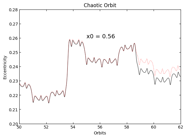
As shown in Fig. 9.8, deviation starts around 60 Jupiter orbits.

# plot the a,e for 4 particles in 2 different location
fig, (ax1, ax2) = plt.subplots(2, 2, figsize=(11, 8))

ax1[0].plot(times / p_orb, tp_a[0], 
         linewidth = 0.7, color = "black", alpha  =1)
ax2[0].plot(times / p_orb, tp_e[0], 
         linewidth = 0.7, color = "black", alpha  =1)
ax1[0].plot(times / p_orb, tp_a[1], 
         linewidth = 0.7, linestyle = "--", color = "red", alpha  =0.5)
ax2[0].plot(times / p_orb, tp_e[1], 
         linewidth = 0.7, linestyle = "--", color = "red", alpha  =0.5)

ax1[0].set_ylabel("a")
ax2[0].set_ylabel("e")
ax2[0].set_xlabel("Orbits")
ax1[1].plot(times / p_orb, tp_a[2], 
         linewidth = 0.7, color = "black", alpha  =1)
ax2[1].plot(times / p_orb, tp_e[2], 
         linewidth = 0.7, color = "black", alpha  =1)

ax1[1].plot(times / p_orb, tp_a[3], 
         linewidth = 0.7, linestyle = "--", color = "red", alpha  =0.5)
ax2[1].plot(times / p_orb, tp_e[3], 
         linewidth = 0.7, linestyle = "--", color = "red", alpha  =0.5)

ax1[1].set_ylabel("a")
ax2[1].set_ylabel("e")
ax2[1].set_xlabel("Orbits")
ax1[0].text(200, 0.995*np.max([tp_a[0], tp_a[1]]), f"x0 = {x0_pack[0]}", fontsize =14)
ax1[1].text(200, 0.995*np.max([tp_a[2], tp_a[3]]), f"x0 = {x0_pack[2]}", fontsize =14)
plt.show()



# to show the divergence of orbit in the second one
fig01, ax3 = plt.subplots(1, 1, figsize=(7, 5))
ax3.set_title("Chaotic Orbit")
ax3.plot(times / p_orb, tp_e[2], 
         linewidth = 0.7, color = "black", alpha  =1)
ax3.plot(times / p_orb, tp_e[3], 
         linewidth = 0.7, linestyle = "--", color = "red", alpha  =0.5)
ax3.set_ylabel("Eccentricity")
ax3.set_xlabel("Orbits")
ax3.set_ylim(0.2, 0.28)
ax3.set_xlim(50, 62)
ax3.text(55, 0.26, f"x0 = {x0_pack[2]}", fontsize =14)
plt.show()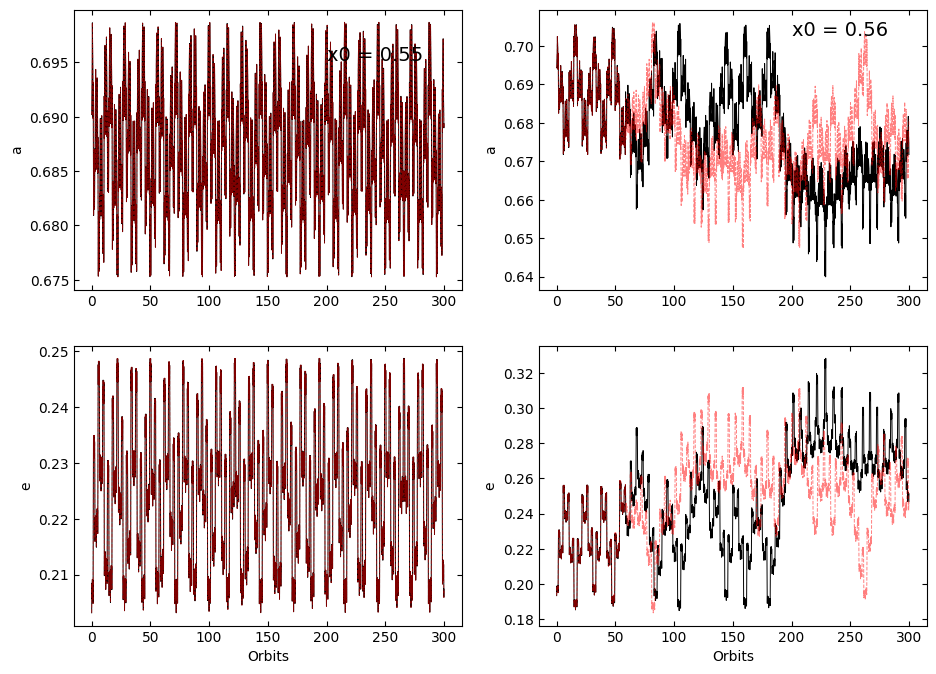

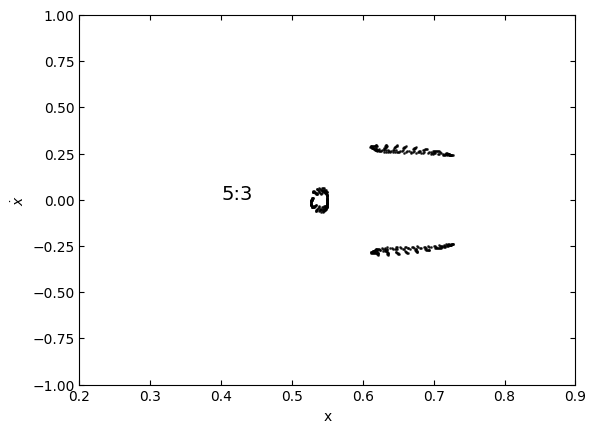
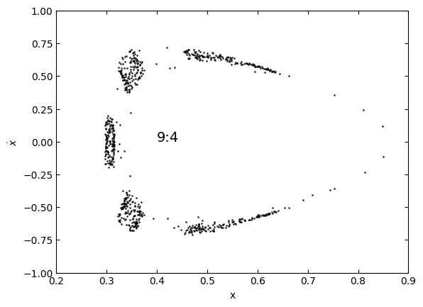
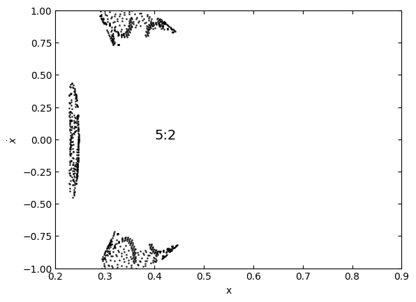
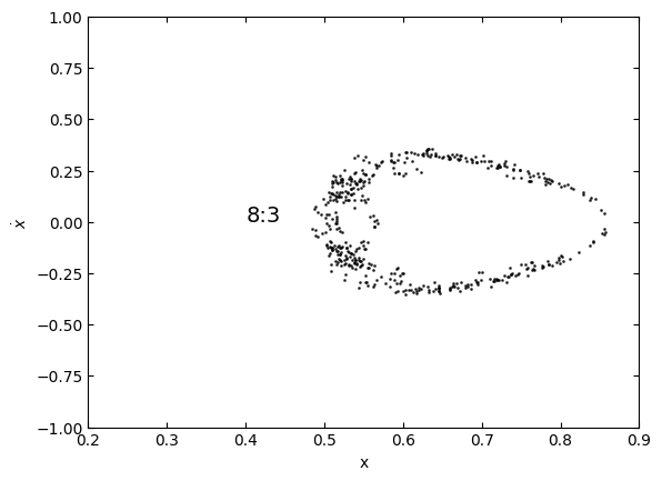
We can see three “islands” in the plot for regular orbits. This is because the orbit is close to the 4:7 resonance orbit with Jupiter.

tp_x_rot = np.zeros((4, Noutputs))
tp_y_rot = np.zeros((4, Noutputs))


fig, ax = plt.subplots(2, 2, figsize=(11, 8))

for i in range(4):
    tp_x_rot[i], tp_y_rot[i] = to_rot_frame(tp_x[i], tp_y[i], ang_p)

    zero_crossings = np.where(np.diff(np.sign(tp_y_rot[i])))[0]

    tp_dxdt = np.gradient(tp_x_rot[i], times)
    tp_dydt = np.gradient(tp_y_rot[i], times)


    dxdt = 0.5*(tp_dxdt[zero_crossings + 1] + tp_dxdt[zero_crossings])
    x    = 0.5*(tp_x_rot[i][zero_crossings + 1] + tp_x_rot[i][zero_crossings])

    ax[i//2][i%2].scatter(x, dxdt, s=1, alpha = 0.7, color = "black")
    ax[i//2][i%2].text(0.65, 0, f"x0={x0_pack[i]}", fontsize = 14)
    ax[i//2][i%2].set_xlim(xmin = 0.45, xmax= 0.9)
    ax[i//2][i%2].set_ylim(ymin = -0.4, ymax= 0.4)


plt.xlabel("x")
plt.ylabel(r"$\dot{x}$")
plt.show()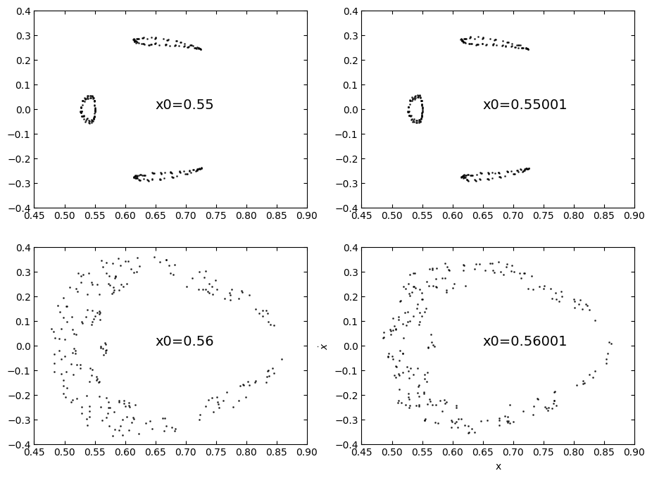

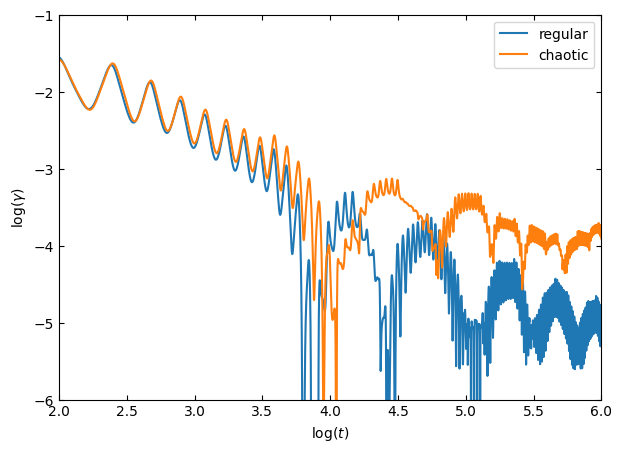
# now we plot the Lyapounov Characteristic: gamma
d0    = 0.00001
di    = np.zeros((2, Noutputs))
gamma = np.zeros((2, Noutputs))

tp_vx_rot =  np.zeros((4, Noutputs))
tp_vy_rot =  np.zeros((4, Noutputs))

def velo_to_rot_frame(zeta, eta, dzeta, deta, l):
    x = np.cos(l)*zeta + np.sin(l)*eta
    y = -np.sin(l)*zeta + np.cos(l)*eta
    xdot = y + np.cos(l)*dzeta + np.sin(l)*deta
    ydot = -x -np.sin(l)*dzeta + np.cos(l)*deta
    return np.array([xdot, ydot])


for j in range(4):
    tp_vx_rot[j], tp_vy_rot[j] = velo_to_rot_frame(tp_x[j], tp_y[j], tp_vx[j], tp_vy[j], ang_p)


di[0] = np.sqrt((tp_x_rot[0] - tp_x_rot[1])**2 + (tp_y_rot[0] - tp_y_rot[1])**2 + 
         (tp_vx_rot[0] - tp_vx_rot[1])**2 + (tp_vy_rot[0] - tp_vy_rot[1])**2)
di[1] = np.sqrt((tp_x_rot[2] - tp_x_rot[3])**2 + (tp_y_rot[2] - tp_y_rot[3])**2 + 
         (tp_vx_rot[2] - tp_vx_rot[3])**2 + (tp_vy_rot[2] - tp_vy_rot[3])**2)


log_did0 = np.log(di[:, 1:]/di[:, :-1])
new_times = times[1:]
# new_times[0] = times[1]

# for j in range(Noutputs):
#     gamma[0][j] = np.sum(log_did0[0][j]) /new_times[j] 
#     gamma[1][j] = np.sum(log_did0[1][j]) /new_times[j]

for j in range(Noutputs-1):
    gamma[0][j+1] = np.sum(log_did0[0][:j]) /new_times[j] 
    gamma[1][j+1] = np.sum(log_did0[1][:j]) /new_times[j]


fig, ax = plt.subplots(1, 1, figsize=(7, 5))
ax.plot(np.log(new_times), np.log(gamma[0][1:]), label = "regular")
ax.plot(np.log(new_times), np.log(gamma[1][1:]), label = "chaotic")
# ax.set_xscale("log")
# ax.set_yscale("log")
ax.set_xlim(xmin=2, xmax = 6)
ax.set_ylim(ymin=-6, ymax = -1)

ax.set_xlabel(r"$\log(t)$")
ax.set_ylabel(r"$\log(\gamma)$")
plt.legend()
plt.show()

/tmp/ipykernel_5494/784641199.py:41: RuntimeWarning: divide by zero encountered in log
  ax.plot(np.log(new_times), np.log(gamma[0][1:]), label = "regular")
/tmp/ipykernel_5494/784641199.py:41: RuntimeWarning: invalid value encountered in log
  ax.plot(np.log(new_times), np.log(gamma[0][1:]), label = "regular")
/tmp/ipykernel_5494/784641199.py:42: RuntimeWarning: divide by zero encountered in log
  ax.plot(np.log(new_times), np.log(gamma[1][1:]), label = "chaotic")
/tmp/ipykernel_5494/784641199.py:42: RuntimeWarning: invalid value encountered in log
  ax.plot(np.log(new_times), np.log(gamma[1][1:]), label = "chaotic")

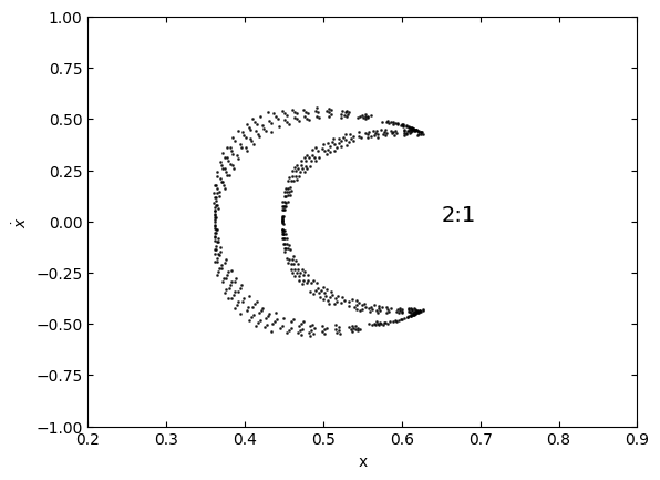
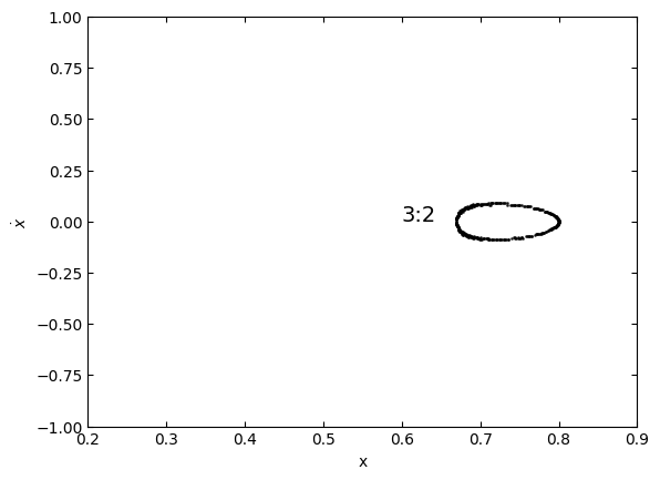
Now, we can use different orbital resonance ratio to create plot with different numbers of “islands”!

# extra part: can we see different resonance cricles?

# for a given x0, cj, we can run a simulation and plot 
def run_one_plot(x0, CJ, norb=600, 
                 note="unknown", loc = [0,0],
                 plot = True):
    a000,  e000,  vx000,  vy000  = get_ae_from_x0(x0, Cj = CJ)

    # setup simulations
    sim = rebound.Simulation()
    sim.add(m = mu1, hash = "star")
    sim.add(m = mu2, a = 1, hash = "jupiter")

    sim.move_to_com()
    # sim.add(m=0, a=a000, e=e000, hash = "loc1")
    sim.add(m=0, x=x0, y=0, vx=vx000, vy=vy000, hash = "loc1")

    num_orb  = norb
    Noutputs = 180*num_orb
    times    = np.linspace(0, num_orb*2*np.pi, Noutputs)

    tp_x = np.zeros(Noutputs)
    tp_y = np.zeros(Noutputs)

    ang_p = np.zeros(Noutputs)

    for i, t in enumerate(times):
        sim.integrate(t, exact_finish_time=1)
        tp_x[i] = sim.particles[2].x
        tp_y[i] = sim.particles[2].y
        orb_p = sim.particles["jupiter"].orbit(primary = sim.particles["star"])
        ang_p[i] = orb_p.theta

    # change to the rotating frame
    tp_x_rot, tp_y_rot = to_rot_frame(tp_x, tp_y, ang_p)

    zero_crossings = np.where(np.diff(np.sign(tp_y_rot)))[0]

    tp_dxdt = np.gradient(tp_x_rot, times)
    dxdt    = 0.5*(tp_dxdt[zero_crossings + 1] + tp_dxdt[zero_crossings])
    x       = 0.5*(tp_x_rot[zero_crossings + 1] + tp_x_rot[zero_crossings])

    if plot == True:
        plt.scatter(x, dxdt, s=1, alpha = 0.7, color = "black")
        plt.text(loc[0], loc[1],  note, fontsize = 14)
        plt.xlim(xmin = 0.2, xmax= 0.9)
        plt.ylim(ymin = -1, ymax= 1)


        plt.xlabel("x")
        plt.ylabel(r"$\dot{x}$")
        plt.show()

    return x, dxdt



# 2:1 resonance:
a0000 = (1/2)**(2/3)
print("for 8:3 orbit, your a0 is:", a0000)
_, _ = run_one_plot(0.448, 3.07, note="2:1", loc = [0.65, 0])
# run_one_plot(0.518, 3.13, note="2:1", loc = [0.65, 0])

for 8:3 orbit, your a0 is: 0.6299605249474366
for the value of x0: 0.448
you get: 0.6513279775947113 0.31063916268711217

# 3:2
run_one_plot(0.8, 3.07, note="3:2", loc = [0.6, 0])

for the value of x0: 0.8
you get: 0.7448072385205545 0.07544604640398452

# 5:3
run_one_plot(0.55, 3.07, note="5:3", loc = [0.4, 0])

for the value of x0: 0.55
you get: 0.6958479821106044 0.2081603824893759

# 9:4
run_one_plot(0.3157, 3.07, note="9:4", loc = [0.4, 0])

for the value of x0: 0.3157
you get: 0.5844553153578788 0.4581279497713602

# 5:2
run_one_plot(0.248, 3.07, note="5:2", loc = [0.4, 0])

for the value of x0: 0.248
you get: 0.5464277234428195 0.5443130183235361

# 8:3
a0000 = (3/8)**(2/3)
print("for 8:3 orbit, your a0 is:", a0000)
run_one_plot(a0000-mu2, 3.07, note="8:3", loc = [0.4, 0])

for 8:3 orbit, your a0 is: 0.520020955762976
for the value of x0: 0.519020955762976
you get: 0.683083476773796 0.23871536430798249

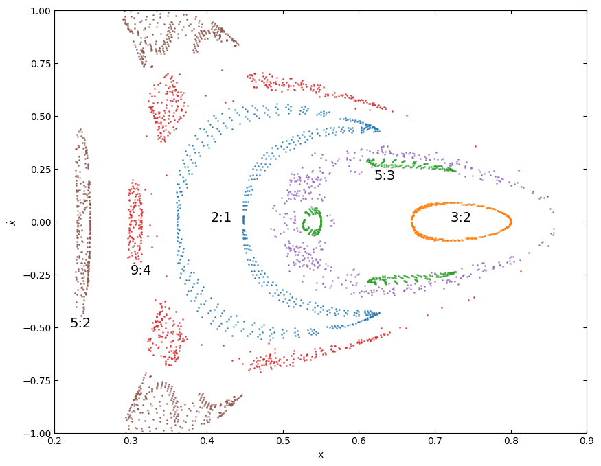
Now, here is all the resonance all together:

x01, dx01 = run_one_plot(0.448, 3.07, note="2:1", plot = False)
x02, dx02 = run_one_plot(0.8, 3.07, note="3:2", plot = False)
x03, dx03 = run_one_plot(0.55, 3.07, note="5:3", plot = False)
x04, dx04 = run_one_plot(0.3157, 3.07, note="9:4", plot = False)
x05, dx05 = run_one_plot((3/8)**(2/3)-mu2, 3.07, note="8:3", plot = False)
x06, dx06 = run_one_plot(0.248, 3.07, note="5:2", plot = False)


fig, ax = plt.subplots(1, 1, figsize=(10, 8))

ax.scatter(x01, dx01, s=1, alpha = 0.7)
ax.scatter(x02, dx02, s=1, alpha = 0.7)
ax.scatter(x03, dx03, s=1, alpha = 0.7)
ax.scatter(x04, dx04, s=1, alpha = 0.7)
ax.scatter(x05, dx05, s=1, alpha = 0.7)
ax.scatter(x06, dx06, s=1, alpha = 0.7)

ax.set_xlim(xmin = 0.2, xmax= 0.9)
ax.set_ylim(ymin = -1, ymax= 1)
ax.set_xlabel("x")

ax.text(0.405, 0, "2:1", color = "black", fontsize = 14)
ax.text(0.3, -0.25, "9:4", color = "black", fontsize = 14)
ax.text(0.72, 0, "3:2", color = "black", fontsize = 14)
ax.text(0.62, 0.2, "5:3", color = "black", fontsize = 14)
ax.text(0.22, -0.5, "5:2", color = "black", fontsize = 14)

ax.set_ylabel(r"$\dot{x}$")
plt.show()

for the value of x0: 0.448
you get: 0.6513279775947113 0.31063916268711217
for the value of x0: 0.8
you get: 0.7448072385205545 0.07544604640398452
for the value of x0: 0.55
you get: 0.6958479821106044 0.2081603824893759
for the value of x0: 0.3157
you get: 0.5844553153578788 0.4581279497713602
for the value of x0: 0.519020955762976
you get: 0.683083476773796 0.23871536430798249
for the value of x0: 0.248
you get: 0.5464277234428195 0.5443130183235361