Week 8 Solutions - PHYS 633 Astrophysical Dynamics

import galpy
from galpy import potential
from galpy.orbit import Orbit
import numpy as np
import matplotlib.pyplot as plt
import rebound

Part 1: Orbits in disks¶

#1

def kepler(ts,R=1.,vT=1.,ro=8.,vo=220.,vR=0.,z=0.,vz=0.,phi=0.):
    pot = potential.KeplerPotential(ro=ro,vo=vo)
    o = Orbit([R,vR,vT,z,vz,phi],ro=ro,vo=vo)
    o.integrate(ts,pot)
    o.plot(d1='x',d2='y')
    plt.gca().set_aspect(1)
    #o.animate(d1='x',d2='y') # UNCOMMENT FOR ANIMATION
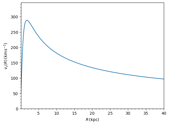
    pot.plotRotcurve()
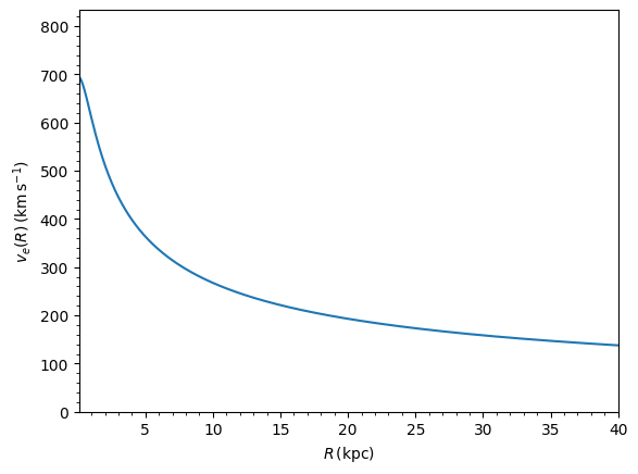
    pot.plotEscapecurve()

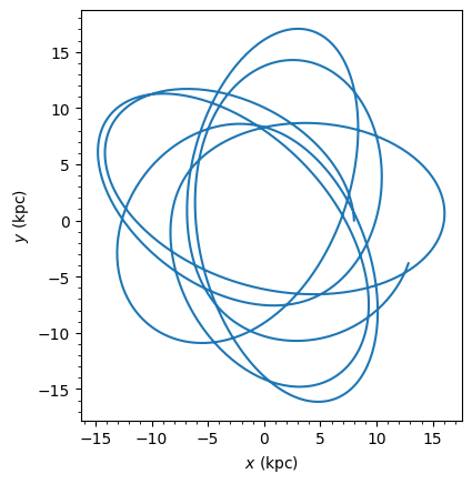
ts = np.linspace(0.,50.,1001)
kepler(ts)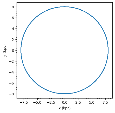

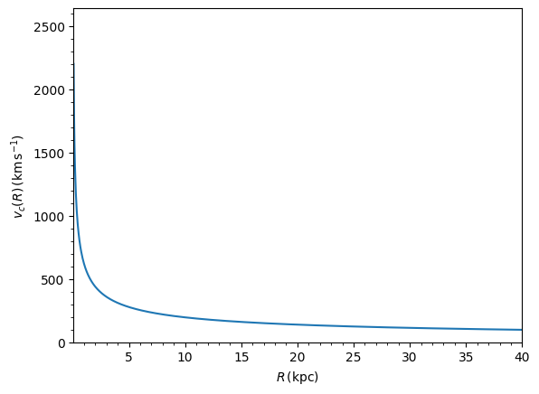
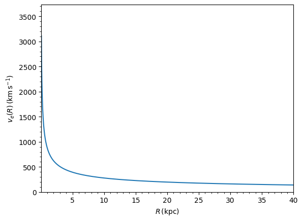
These curves follow a $\frac{1}{r}$ curve, as expected. The orbit remains stable as expected from a point mass potential. We need to have $\frac{GM}{r}=v^2$ in order for the stability. If we change $v_R$ , we get an elliptic orbit with the center of the orbit located at one of the focus of the ellipse. Varying the angle $\phi$ rotates the orbit.

#2

def iso(ts,R=1.,vT=1.,b=.1,ro=8.,vo=220.,vR=0.,z=0.,vz=0.,phi=0.):
    pot = potential.IsochronePotential(b=b,ro=ro,vo=vo)
    o = Orbit([R,vR,vT,z,vz,phi],ro=ro,vo=vo)
    o.integrate(ts,pot)
    o.plot(d1='x',d2='y')
    plt.gca().set_aspect(1)
    #o.animate(d1='x',d2='y') # UNCOMMENT FOR ANIMATION
    pot.plotRotcurve()
    pot.plotEscapecurve()

ts = np.linspace(0.,100.,2001)
iso(ts)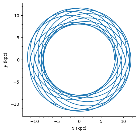

We notice the peak in the rotation curve occurs at $b$ which is represented as a fractional value of $r_o$ . The orbit is elliptical and precesses with time. Setting $b=0$ we get the same results as the point mass potential.

#3

def MW(ts,R,E,Lz,ro=8.,vo=220.,vR=0.,z=0.,phi=0.,contour=True):
    pot = potential.MWPotential2014
    vz = np.sqrt(2 * (E - potential.evaluatePotentials(pot,R,z,phi) - ((Lz/R) ** 2) / 2. - (vR ** 2) / 2))
    vT = Lz / R
    o = Orbit([R,vR,vT,z,vz,phi],ro=ro,vo=vo)
    o.integrate(ts,pot)
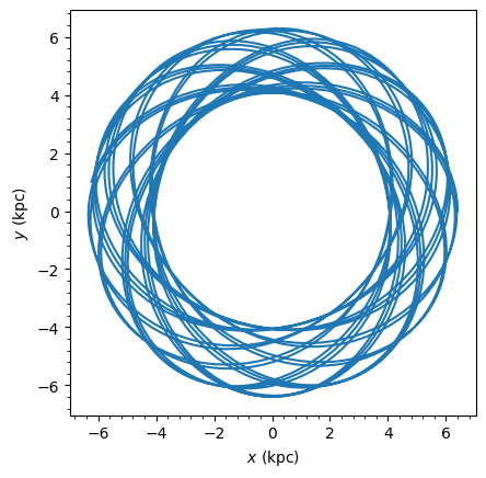
    o.plot(d1='x',d2='y')
    plt.gca().set_aspect(1)
    #o.animate(d1='x',d2='y') # UNCOMMENT FOR ANIMATION
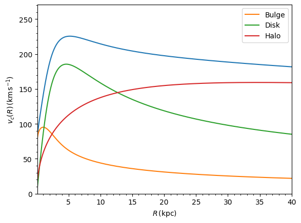
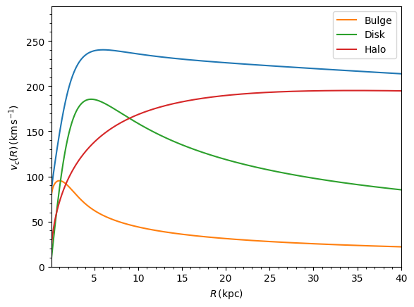
    potential.plotRotcurve(pot,ro=ro,vo=vo)
    pot[0].plotRotcurve(ro=ro,vo=vo,label='Bulge',overplot=True)
    pot[1].plotRotcurve(ro=ro,vo=vo,label='Disk',overplot=True)
    pot[2].plotRotcurve(ro=ro,vo=vo,label='Halo',overplot=True)
    plt.legend()
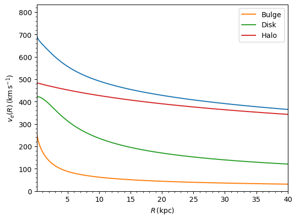
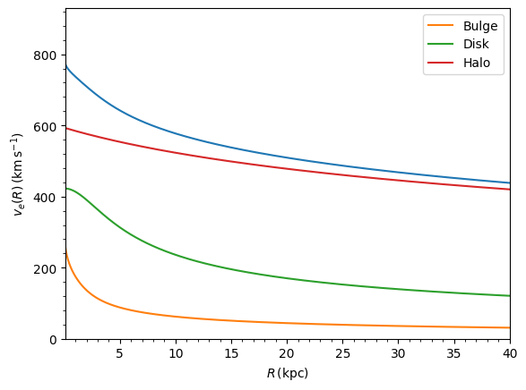
    potential.plotEscapecurve(pot,ro=ro,vo=vo)
    pot[0].plotEscapecurve(ro=ro,vo=vo,label='Bulge',overplot=True)
    pot[1].plotEscapecurve(ro=ro,vo=vo,label='Disk',overplot=True)
    pot[2].plotEscapecurve(ro=ro,vo=vo,label='Halo',overplot=True)
    plt.legend()

    if not contour:
        return

    levels= np.linspace(E,0.,11)
    cntrcolors= ['k' for l in levels]
    cntrcolors[np.arange(len(levels))\
               [np.fabs(levels-E) < 0.01][0]]= '#ff7f0e'
    cntrlw= [1.5 for l in levels]
    cntrlw[np.arange(len(levels))\
               [np.fabs(levels-E) < 0.01][0]]= 5.
    plt.figure(figsize=(10,6))
    potential.plotPotentials(pot,
                             nrs=101,nzs=101,
                             justcontours=True,
                             levels=levels,
                             cntrcolors=cntrcolors,
                             cntrlw=cntrlw,
                             effective=True,
                             Lz=Lz,gcf=True,
                             ro=ro,vo=vo)
    o.plot(overplot=True,lw=0.5)
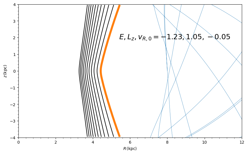
    galpy.util.plot.text(5.4,1.9,
                    r'$E, L_z, v_{R,0}= %.2f, %.2f, %.2f$' % (E,Lz,vR),
                    size=18.)

ts = np.linspace(0.,100.,2001)
MW(ts,.8,-1.25,.6,contour=True)

/home/cumming/projects_local/rebound/rebound-venv/lib/python3.13/site-packages/galpy/potential/PowerSphericalPotentialwCutoff.py:85: RuntimeWarning: invalid value encountered in scalar divide
  - special.gamma(1.5 - self.alpha / 2.0)

/home/cumming/projects_local/rebound/rebound-venv/lib/python3.13/site-packages/galpy/potential/Potential.py:2694: RuntimeWarning: divide by zero encountered in scalar divide
  potRz[ii, :] += 0.5 * Lz**2 / Rs[ii] ** 2.0

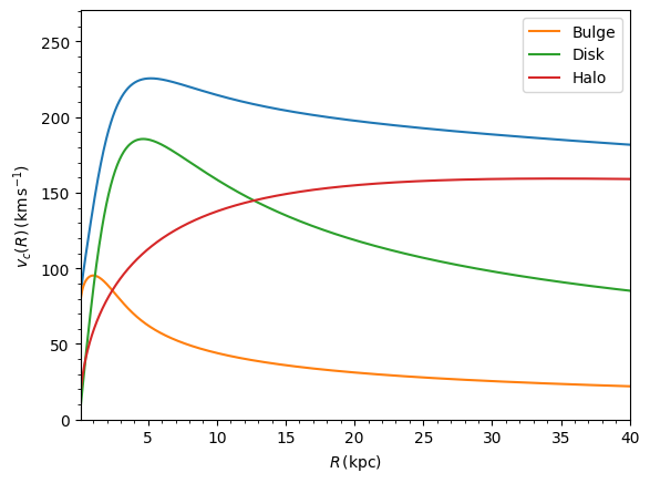
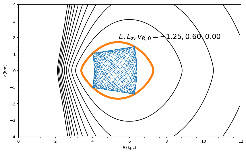
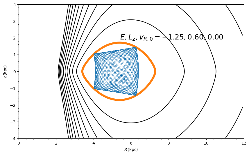
The orbit in the $R-z$ plane is delimited by the contour associated with the intial values of the orbit’s energy, vertical angular momentum, and radial velocity where it intersects at 4 differents positions.

#4

def MW(ts,R,E,Lz,Mbh=4*10**6,ro=8.,vo=220.,vR=0.,z=0.,phi=0.,contour=True):
    pot = potential.MWPotential2014 + potential.KeplerPotential(amp=Mbh/galpy.util.conversion.mass_in_msol(vo=vo,ro=ro))
    vz = np.sqrt(2 * (E - potential.evaluatePotentials(pot,R,z,phi) - ((Lz/R) ** 2) / 2. - (vR ** 2) / 2))
    vT = Lz / R
    o = Orbit([R,vR,vT,z,vz,phi],ro=ro,vo=vo)
    o.integrate(ts,pot)
    o.plot(d1='x',d2='y')
    plt.gca().set_aspect(1)
    #o.animate(d1='x',d2='y') # UNCOMMENT FOR ANIMATION
    potential.plotRotcurve(pot,ro=ro,vo=vo)
    pot[0].plotRotcurve(ro=ro,vo=vo,label='Bulge',overplot=True)
    pot[1].plotRotcurve(ro=ro,vo=vo,label='Disk',overplot=True)
    pot[2].plotRotcurve(ro=ro,vo=vo,label='Halo',overplot=True)
    plt.legend()
    potential.plotEscapecurve(pot,ro=ro,vo=vo)
    pot[0].plotEscapecurve(ro=ro,vo=vo,label='Bulge',overplot=True)
    pot[1].plotEscapecurve(ro=ro,vo=vo,label='Disk',overplot=True)
    pot[2].plotEscapecurve(ro=ro,vo=vo,label='Halo',overplot=True)
    plt.legend()

    if not contour:
        return

    levels= np.linspace(E,0.,11)
    cntrcolors= ['k' for l in levels]
    cntrcolors[np.arange(len(levels))\
               [np.fabs(levels-E) < 0.01][0]]= '#ff7f0e'
    cntrlw= [1.5 for l in levels]
    cntrlw[np.arange(len(levels))\
               [np.fabs(levels-E) < 0.01][0]]= 5.
    plt.figure(figsize=(10,6))
    potential.plotPotentials(pot,
                             nrs=101,nzs=101,
                             justcontours=True,
                             levels=levels,
                             cntrcolors=cntrcolors,
                             cntrlw=cntrlw,
                             effective=True,
                             Lz=Lz,gcf=True,
                             ro=ro,vo=vo)
    o.plot(overplot=True,lw=0.5)
    galpy.util.plot.text(5.4,1.9,
                    r'$E, L_z, v_{R,0}= %.2f, %.2f, %.2f$' % (E,Lz,vR),
                    size=18.)

ts = np.linspace(0.,100.,2001)
MW(ts,.8,-1.25,.6,contour=True)

/home/cumming/projects_local/rebound/rebound-venv/lib/python3.13/site-packages/galpy/potential/Potential.py:2694: RuntimeWarning: invalid value encountered in add
  potRz[ii, :] += 0.5 * Lz**2 / Rs[ii] ** 2.0

#5

def MW(ts,R,E,Lz,Mbh=4*10**6,m=1.,ro=8.,vo=220.,vR=0.,z=0.,phi=0.,contour=True):
    pot = potential.MWPotential2014 + potential.KeplerPotential(amp=Mbh/galpy.util.conversion.mass_in_msol(vo=vo,ro=ro))
    pot[2] *= 1.5
    vz = np.sqrt(2 * (E - potential.evaluatePotentials(pot,R,z,phi) - ((Lz/R) ** 2) / 2. - (vR ** 2) / 2))
    vT = Lz / R
    o = Orbit([R,vR,vT,z,vz,phi],ro=ro,vo=vo)
    #o.integrate(ts,pot)
    o.integrate(pot)
    o.plot(d1='x',d2='y')
    plt.gca().set_aspect(1)
    #o.animate(d1='x',d2='y') # UNCOMMENT FOR ANIMATION
    potential.plotRotcurve(pot,ro=ro,vo=vo)
    pot[0].plotRotcurve(ro=ro,vo=vo,label='Bulge',overplot=True)
    pot[1].plotRotcurve(ro=ro,vo=vo,label='Disk',overplot=True)
    pot[2].plotRotcurve(ro=ro,vo=vo,label='Halo',overplot=True)
    plt.legend()
    potential.plotEscapecurve(pot,ro=ro,vo=vo)
    pot[0].plotEscapecurve(ro=ro,vo=vo,label='Bulge',overplot=True)
    pot[1].plotEscapecurve(ro=ro,vo=vo,label='Disk',overplot=True)
    pot[2].plotEscapecurve(ro=ro,vo=vo,label='Halo',overplot=True)
    plt.legend()

    if not contour:
        return

    levels= np.linspace(E,0.,11)
    cntrcolors= ['k' for l in levels]
    cntrcolors[np.arange(len(levels))\
               [np.fabs(levels-E) < 0.01][0]]= '#ff7f0e'
    cntrlw= [1.5 for l in levels]
    cntrlw[np.arange(len(levels))\
               [np.fabs(levels-E) < 0.01][0]]= 5.
    plt.figure(figsize=(10,6))
    potential.plotPotentials(pot,
                             nrs=101,nzs=101,
                             justcontours=True,
                             levels=levels,
                             cntrcolors=cntrcolors,
                             cntrlw=cntrlw,
                             effective=True,
                             Lz=Lz,gcf=True,
                             ro=ro,vo=vo)
    o.plot(overplot=True,lw=0.5)
    galpy.util.plot.text(5.4,1.9,
                    r'$E, L_z, v_{R,0}= %.2f, %.2f, %.2f$' % (E,Lz,vR),
                    size=18.)
    arr = potential.vesc(pot,o.R(o.time(ro=ro,vo=vo),ro=ro,vo=vo))
    index = np.argmin(arr)
    vesc = min(arr) * vo
    print(f"The smallest escape velocity occurring within 10 dynamical times is {vesc} km/s.")
    m = m * 1.989e30
    eesc = (1 / 2) * m * (vesc * 1e3) ** 2 - o.E(t=o.time(ro=ro,vo=vo)[index],pot=pot,vo=vo) * m
    print(f"The energy required for the Sun to escape the Milky Way potential with a higher estimate in DM is {eesc} J.")

ts = np.linspace(0.,100.,2001)
MW(ts,1.,-1.23,232/220,vR=-11/220,contour=True)

The smallest escape velocity occurring within 10 dynamical times is 348.6085792888689 km/s.
The energy required for the Sun to escape the Milky Way potential with a higher estimate in DM is 1.208596562844055e+41 J.

#6

def MW(ts,R,E,Lz,Mbh=4*10**6,m=1.,ro=8.,vo=220.,vR=0.,z=0.,phi=0.,contour=True):
    pot = potential.MWPotential2014 #+ potential.KeplerPotential(amp=Mbh/galpy.util.conversion.mass_in_msol(vo=vo,ro=ro))
    #pot[2] *= 1.5
    vz = np.sqrt(2 * (E - potential.evaluatePotentials(pot,R,z,phi) - ((Lz/R) ** 2) / 2. - (vR ** 2) / 2))
    vT = Lz / R
    o = Orbit([R,vR,vT,z,vz,phi],ro=ro,vo=vo)
    o.integrate(ts,pot)
    olin = o.toLinear()
    oplanar = o.toPlanar()
    #o.plot(d1='x',d2='y')
    #plt.gca().set_aspect(1)
    #o.animate(d1='x',d2='y') # UNCOMMENT FOR ANIMATION
    

    if not contour:
        return
        
    

ts = np.linspace(0.,100.,10001)
MW(ts,.8,-1.25,.6,contour=True)

Part 2: Geometry of Resonances¶

# 7

def rotate(x, y, theta, n):
    return [x * np.cos(n * theta) + y * np.sin(n * theta), -x * np.sin(n * theta) + y * np.cos(n * theta)]

mu2 = 0 # common mistake to reproduce the plot is taking this value (albeit more realistic): 1e-3
# p : q where p for test mass and q for Jupiter
p = 5
q = 3
n = p / q
T = 2 * np.pi
sim = rebound.Simulation()
sim.add(m=1.0-mu2, hash="Sun")
sim.add(m=mu2, P=T, e=0.0, hash="Jupiter")
sim.move_to_com()
sim.add(m=0.0, P=T/n, e=.3, hash="Test")

Noutputs = 200
Norbits = q
times = np.linspace(0, Norbits * T, Noutputs)

xy = np.zeros((Noutputs, 3, 2))
xy_r = np.zeros((Noutputs, 3, 2))

for i,t in enumerate(times):
    sim.integrate(t, exact_finish_time=1)
    xy[i][0] = [sim.particles["Sun"].x, sim.particles["Sun"].y]
    xy[i][1] = [sim.particles["Jupiter"].x, sim.particles["Jupiter"].y]
    xy[i][2] = [sim.particles["Test"].x, sim.particles["Test"].y]

    orb = sim.particles["Jupiter"].orbit(primary=sim.particles["Sun"])
    
    theta = orb.theta
    
    xy_r[i][0] = rotate(xy[i][0][0], xy[i][0][1], theta, 1)
    xy_r[i][1] = rotate(xy[i][1][0], xy[i][1][1], theta, 1)
    xy_r[i][2] = rotate(xy[i][2][0], xy[i][2][1], theta, 1)

plt.plot(xy_r[:,2,0], xy_r[:,2,1], label="Test particle")
plt.scatter(xy_r[0,0,0], xy_r[0,0,1], color="r", label="Sun")
plt.scatter(xy_r[0,1,0], xy_r[0,1,1], color="g", label="Jupiter")
plt.legend()
plt.ylim(-1.5,1.5)
plt.xlim(-1.5,1.5)
plt.show()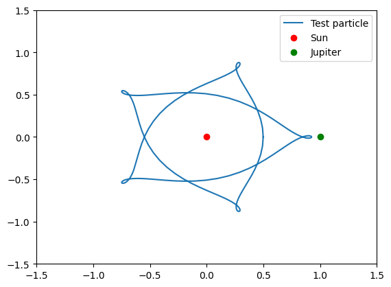

When adding a mass to Jupiter,the expected orbits do not fully close even when we have $p:q$ resonance after $q$ orbits. This is related to the restricted three body problem. For a given $p:q$ with $m_J=0$ , we’d have to change the parameters of the orbit in order to obtain similar results.