Reading questions
What is the difference between collisionless and collisional systems? Strong gravitational interactions between individual stars dominate the evolution of a collisional system, whereas they are are negligible in a collisionless system.
(a) What are the relaxation time and dynamical time of a galaxy? (b) How can one argue that galaxies are collisionless, by comparing their two-body relaxation time with the age of the Universe? (a) The relaxation time of a galaxy is the time required to change one of its star’s velocity by 100%. The dynamical time of a galaxy is the crossing time for individual stars. The crossing time is where is the galaxy size and is the velocity of the star. We also have that the relaxation time is , where , where is the number of stars in the galaxy. (b) For a typical galaxy, we have and . This yields , or 5 million times the age of our Universe. This means that two-body relaxation cannot be the mechanism through which galaxies reach dynamical equilibrium; otherwise, they would be far from equilibrium today.
(a) What’s the assumption required for dynamical equilibrium, based on the virial theorem? (b) Under this assumption, what is the relation between kinetic and potential energy? (a) The fundamental assumption of the virial theorem is that the system is in equilibrium, e.g. that , where is the virial quantity and is defined as , where are arbitrary weights and and are the position and velocity of the -th particle, respectively. (b) With this assumption, the result of the virial theorem is that , where is the kinetic energy of the system and is its gravitational potential energy.
What is the collisionless Boltzmann equation? The collisionless Boltzmann equation is:
where is the distribution function of the system. The collisionless Boltzmann equation describes the behavior of under the influence of gravity.
What are the Jeans equations, and what applicability do they have for studying astronomical systems of many objects? Jeans equations are the collisionless Boltzmann equation multiplied by powers of or and integrated over a part of phase-space. They are moment equations of the collisionless Boltzmann equation. They are useful in astronomy because astronomical observations are usually performed at a fixed location in the sky. Thus, multiplying the collisionless Boltzmann equation by v and integrating over all components of the velocity connects to observables.
Numerical Exercise
In this exercise, we will use to investigate the gravitational potential of dark matter profiles in dwarf galaxies using the Jeans equations formulation for collisionless systems. We will use mock data based on Walker et al. (2009) https://
import matplotlib.pyplot as plt
import time
import numpy as np
import galpy
from galpy.df import jeans
Select one of the dwarf galaxies data for line-of-sight (LOS) velocity dispersion profiles. The columns are (1) radial distance in the plane of the sky in pc, (2) LOS velocity dispersion measured at the given radial distance in km/s, (3) error in the velocity dispersion measured in km/s
These values might be useful since galpy standard units are given in velocity normalized by the circular velocity of the Milky Way , and the approximate distance of the sun to the Milky Way’s center .
v0=220 #km/s
r0=8e3 #pc
G_c=4.30091e-3 #pc (km/s)^2 Msun^-1
In Walker et al. (2009) two of the dark matter profiles that are studied are the Navarro–Frenk–White (NFW) profile https://
We can define a potential we are working with in galpy as follows (NFW as example): (giving ro and vo will produce outputs in for densities and for velocity dispersions, inputs must be on galpy units though).
To explore the dark matter profile of dwarf galaxies, we will use the density profiles that define the potential with a characteristic density . Such a density will be the input in our potentials (for the NFW profile as defined in you might want to write ). Density inputs have units
(1) After selecting one of the galaxies, define an NFW and Burkert potential in and plot the corresponding density profiles in a range of 10 to 2000 pc. Taking the previous example, you can use to evaluate the density of the given potential at different distances . Use at least 3 values of scale density in the range - for each profile. What are the main differences between the two density distributions (you might use a log scale in your plots).
rho0=np.array([0.01,0.05,5])/((v0**2)/(G_c*(r0**2)))
nfwr0=795/r0 # Normalized by 8kpc
core0=150/r0#Normalized by 8kpc

rho02=np.array([0.02,1,10])/((v0**2)/(G_c*(r0**2)))
NFW1=galpy.potential.NFWPotential(amp=rho0[0]*4*np.pi*(nfwr0**3), a=nfwr0,vo=v0, ro=r0/1e3)
NFW2=galpy.potential.NFWPotential(amp=rho0[1]*4*np.pi*(nfwr0**3), a=nfwr0,vo=v0, ro=r0/1e3)
NFW3=galpy.potential.NFWPotential(amp=rho0[2]*4*np.pi*(nfwr0**3), a=nfwr0,vo=v0, ro=r0/1e3)
core1=galpy.potential.BurkertPotential(amp=rho02[0], a=core0,vo=v0, ro=r0/1e3)
core2=galpy.potential.BurkertPotential(amp=rho02[1], a=core0,vo=v0, ro=r0/1e3)
core3=galpy.potential.BurkertPotential(amp=rho02[2], a=core0,vo=v0, ro=r0/1e3)rr=np.geomspace(20,2000,100)/r0import matplotlib
matplotlib.use('TkAgg')%matplotlib inlineplt.loglog(rr*r0,NFW1.dens(rr,0),label=r'NFW, $\rho_{0}=0.01 \ \mathrm{M_{\odot}\ pc^{-3}}$')
plt.loglog(rr*r0,NFW2.dens(rr,0),label=r'NFW, $\rho_{0}=0.05 \ \mathrm{M_{\odot}\ pc^{-3}}$')
plt.loglog(rr*r0,NFW3.dens(rr,0),label=r'NFW, $\rho_{0}=5 \ \mathrm{M_{\odot}\ pc^{-3}}$')
plt.loglog(rr*r0,core1.dens(rr,0),label=r'core, $\rho_{0}=0.02 \ \mathrm{M_{\odot}\ pc^{-3}}$')
plt.loglog(rr*r0,core2.dens(rr,0),label=r'core, $\rho_{0}=1 \ \mathrm{M_{\odot}\ pc^{-3}}$')
plt.loglog(rr*r0,core3.dens(rr,0),label=r'core, $\rho_{0}=10 \ \mathrm{M_{\odot}\ pc^{-3}}$')
plt.xlabel('r (pc)')
plt.ylabel(r'$\rho \ (\mathrm{M_{\odot} pc^{-3}}$)')
plt.legend()
plt.show()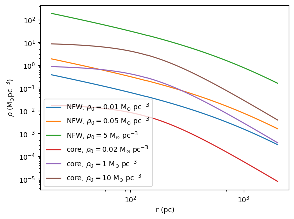
(2) Since we only have access to LOS velocities, we need the anisotropy to compute the velocity dispersions from the Jeans equations. Use at least 5 values of the anisotropy in the range -1 and compute the radial velocity dispersions with . Use to compute at a given radial distance . Plot vs (do not compare with the data yet).
beta=np.array([-5,-0.5,0,0.5,1])sigs1=[]
sigs2=[]
sigs3=[]
sigs1_=[]
sigs2_=[]
sigs3_=[]
for i in beta:
sig1=np.array([jeans.sigmar(NFW1,r,beta=i) for r in rr])/v0
sigs1.append(sig1)
sig2=np.array([jeans.sigmar(NFW2,r,beta=i) for r in rr])/v0
sigs2.append(sig2)
sig3=np.array([jeans.sigmar(NFW3,r,beta=i) for r in rr])/v0
sigs3.append(sig3)
sig1_= np.array([jeans.sigmar(core1,r,beta=i) for r in rr])/v0
sigs1_.append(sig1_)
sig2_= np.array([jeans.sigmar(core2,r,beta=i) for r in rr])/v0
sigs2_.append(sig2_)
sig3_= np.array([jeans.sigmar(core3,r,beta=i) for r in rr])/v0
sigs3_.append(sig3_)
f,ax=plt.subplots(3,1,figsize=(5,10))
for i in range(5):
    ax[0].semilogy(rr*r0,sigs1[i],label=r'$\beta=$'+str(beta[i]))
    ax[1].semilogy(rr*r0,sigs2[i],label=r'$\beta=$'+str(beta[i]))
    ax[2].semilogy(rr*r0,sigs3[i],label=r'$\beta=$'+str(beta[i]))

for i in range(3):
    ax[i].set_xlabel('r (pc)')
    ax[i].set_ylabel(r'$\sigma_{r}\ (\mathrm{km/s}$)')
    ax[i].legend()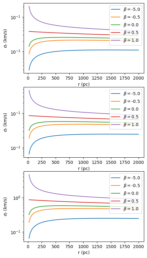
f,ax=plt.subplots(3,1,figsize=(5,10))
for i in range(5):
    ax[0].semilogy(rr*r0,sigs1_[i],label=r'$\beta=$'+str(beta[i]))
    ax[1].semilogy(rr*r0,sigs2_[i],label=r'$\beta=$'+str(beta[i]))
    ax[2].semilogy(rr*r0,sigs3_[i],label=r'$\beta=$'+str(beta[i]))
for i in range(3):
    ax[i].set_xlabel('r (pc)')
    ax[i].set_ylabel(r'$\sigma_{r}\ (\mathrm{km/s}$)')
    ax[i].legend()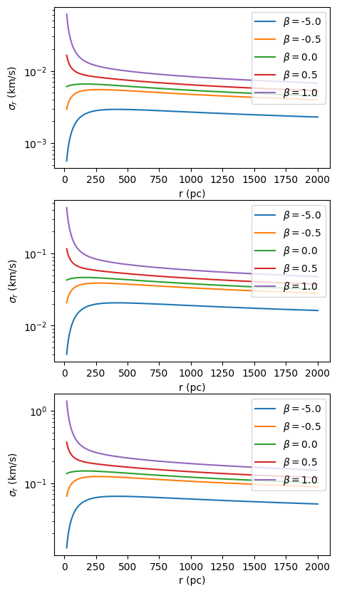
(3) is defined in an arbitrary radial position of the sky, contains information about the inclination of our system, and then it can be used to obtain projected that we can compare with our data. Use to compute at given distances. The densities of stars (dens) and (surfdens) should be functions of (use ), you can use the analytical formulas given in section 3.1 of Walker et al. (2009), note that can be ignored and Table 1 lists the for each galaxy. Plot the obtained with the different values of and for the two dark matter profiles and compare with your data.
a=221/r0 #half radius (pc) /r0def nu(r):
"""3D Plummer tracer density"""
return 3*((4*np.pi*(a**3))**-1)*((1 + r**2 / a**2)**(-5/2))
def I(r):
"""Projected Plummer surface density"""
return ((np.pi*(a**2))**(-1))*((1 + r**2 / a**2)**(-2))sigs_losp1=[]
sigs_losp2=[]
sigs_losp3=[]
sigs_losp1_=[]
sigs_losp2_=[]
sigs_losp3_=[]
for i in range(len(beta)):
#for j in range(len(5)):
#sig1=numpy.array([jeans.sigmar(NFW1,r,beta=i) for r in rr])/v0
sig_losp1=np.array([jeans.sigmalos(NFW1,rr[j],dens=nu,surfdens=I,beta=beta[i],sigma_r=sigs1[i][j]) for j in range(len(sigs1[i]))])
sigs_losp1.append(sig_losp1)
sig_losp2=np.array([jeans.sigmalos(NFW2,rr[j],dens=nu,surfdens=I,beta=beta[i],sigma_r=sigs2[i][j]) for j in range(len(sigs2[i]))])
sigs_losp2.append(sig_losp2)
sig_losp3=np.array([jeans.sigmalos(NFW3,rr[j],dens=nu,surfdens=I,beta=beta[i],sigma_r=sigs3[i][j]) for j in range(len(sigs3[i]))])
sigs_losp3.append(sig_losp3)
sig_losp1_=np.array([jeans.sigmalos(core1,rr[j],dens=nu,surfdens=I,beta=beta[i],sigma_r=sigs1_[i][j]) for j in range(len(sigs1[i]))])
sigs_losp1_.append(sig_losp1_)
sig_losp2_=np.array([jeans.sigmalos(core2,rr[j],dens=nu,surfdens=I,beta=beta[i],sigma_r=sigs2_[i][j]) for j in range(len(sigs2[i]))])
sigs_losp2_.append(sig_losp2_)
sig_losp3_=np.array([jeans.sigmalos(core3,rr[j],dens=nu,surfdens=I,beta=beta[i],sigma_r=sigs3_[i][j]) for j in range(len(sigs3[i]))])
sigs_losp3_.append(sig_losp3_)dr_data=np.loadtxt('draco_walker2009.csv',skiprows=1,delimiter=',', unpack=True)f,ax=plt.subplots(3,1,figsize=(5,10))
for i in range(5):
ax[0].semilogy(rr*r0,sigs_losp1[i],label=r'$\beta=$'+str(beta[i]))
ax[1].semilogy(rr*r0,sigs_losp2[i],label=r'$\beta=$'+str(beta[i]))
ax[2].semilogy(rr*r0,sigs_losp3[i],label=r'$\beta=$'+str(beta[i]))
for i in range(3):
ax[i].errorbar(dr_data[0],dr_data[1],yerr=dr_data[2],fmt='o')
ax[i].set_xlabel('r (pc)')
ax[i].set_ylabel(r'$\sigma_{\mathrm{LOS}}\ (\mathrm{km/s}$)')
ax[i].legend()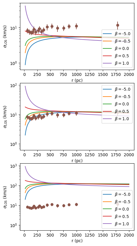
f,ax=plt.subplots(3,1,figsize=(5,10))
for i in range(5):
    ax[0].semilogy(rr*r0,sigs_losp1_[i],label=r'$\beta=$'+str(beta[i]))
    ax[1].semilogy(rr*r0,sigs_losp2_[i],label=r'$\beta=$'+str(beta[i]))
    ax[2].semilogy(rr*r0,sigs_losp3_[i],label=r'$\beta=$'+str(beta[i]))

for i in range(3):
    ax[i].errorbar(dr_data[0],dr_data[1],yerr=dr_data[2],fmt='o')
    ax[i].set_xlabel('r (pc)')
    ax[i].set_ylabel(r'$\sigma_{\mathrm{LOS}}\ (\mathrm{km/s}$)')
    ax[i].legend()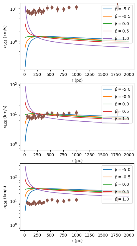
(4) Select your best model to compute the total mass of dark matter contained in a radius of 300 pc and of your selected galaxy and compare with Table 2 of Walker et al. (2009).
plt.plot(rr*r0,sigs_losp2[0],label=r'NFW, $\beta=-5,\ \rho_{0}=0.05 \ \mathrm{M_{\odot}\ pc^{-3}}$')
plt.plot(rr*r0,sigs_losp2_[1],label=r'core, $\beta=-1,\ \rho_{0}=1 \ \mathrm{M_{\odot}\ pc^{-3}}$')
plt.errorbar(dr_data[0],dr_data[1],yerr=dr_data[2],fmt='o')
plt.xlabel('r (pc)')
plt.ylabel(r'$\sigma_{\mathrm{LOS}}\ (\mathrm{km/s}$)')
plt.legend()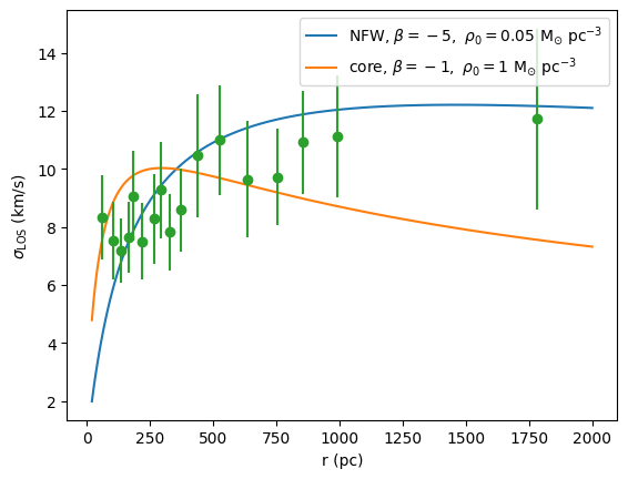
import scipy.integrate as sidef mass_NFW(r):
return 4*np.pi*NFW2.dens(r/r0,0)*(r**2)
def mass_core(r):
return 4*np.pi*core2.dens(r/r0,0)*(r**2) si.quad(mass_NFW,0,300,points=300)[0]/1e7,si.quad(mass_NFW,0,a*r0,points=300)[0]/1e7 #in 10^7 Msun(1.4583937189357992, 0.8766107602579909)si.quad(mass_core,0,300,points=300)[0]/1e7,si.quad(mass_core,0,a*r0,points=300)[0]/1e7 #in 10^7 Msun(1.688361941247572, 1.077373655671226)