#%matplotlib widget
%config InlineBackend.figure_format = 'retina'
import matplotlib.pyplot as plt
import rebound
import time
import numpy as np
Reading questions
(a) is referred to as a pseudo-potential because it includes the centrifugal term which is frame-dependent (only exists in the rotating frame). It also doesn’t describe the full acceleration of the particle because it doesn’t include the Coriolis force.
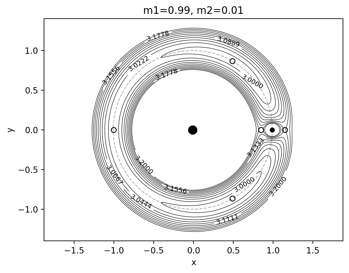
(b) The contours shown in the Figs. 3.7 and 3.9 are zero-velocity curves, which are contours of the Jacobi constant evaluated with . Since , they are equivalent to contours of the pseudo-potential . Ignoring the Coriolis force, the acceleration of the particle is , so the contours show you how the particle would accelerate at any given point if it had zero velocity (so Coriolis vanishes). The Lagrange points are equlibrium points where the gravitational and centrifugal forces balance, and correspond to maxima of , as shown in Figure 3.8.
(c) Looking at Fig. 3.8, we can see that the Lagrange points are all unstable, at least in one direction (saddle points) (since this figure plots , particles want to flow downhill in this plot). So if it were not for the Coriolis force, small displacements away from the Lagrange points would grow, particles would move away from them, they are unstable (see Fig 3.11 which shows the accelerations near the L4 point). However, this neglects Coriolis forces which when included stabilize motions near the L4 and L5 points as long as the mass ratio is small enough - (eq. 3.145). The L1,L2,L3 points on the other hand are always unstable -- although see the comment on p92 at the end of section 3.7.1 which says that you can find some stable orbits, e.g. SOHO’s orbit near L1.
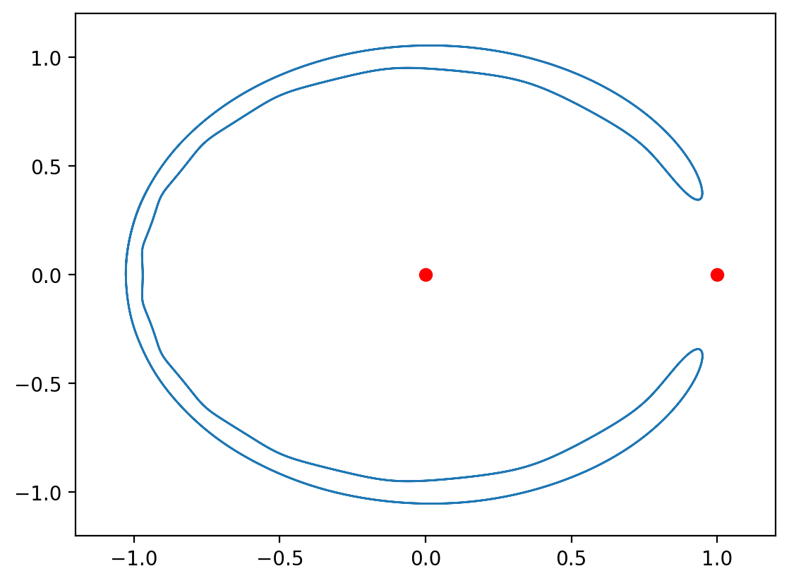
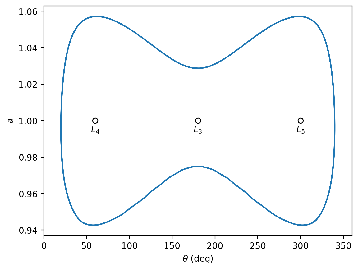
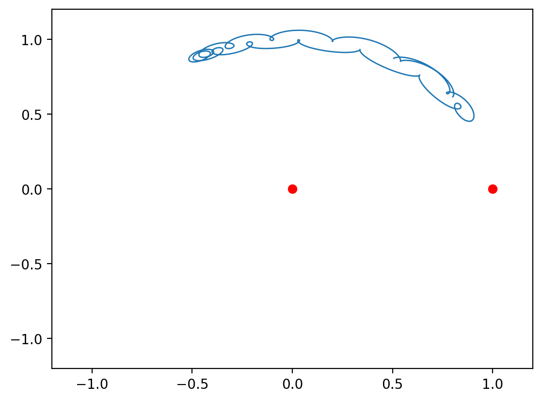
(d) The motions near L4 and L5 are classified into tadpole and horseshoe orbits. In tadpole orbits, the motion librates around one of the Lagrange points, whereas in horseshoe orbits, the particle moves from L4 to L5 and back, as seen in Fig. 3.18.
(e) The Hill sphere is the region around a planet where the planet’s gravity dominates the tidal force from the companion. It corresponds to the region within the L1 and L2 points where the zero-velocity contours become circular.
Part (a)
def zerov_contours(m2,levels):
    m1 = 1-m2
    x = np.linspace(-1.8, 1.8, 400)
    y = np.linspace(-1.8, 1.8, 400)
    X, Y = np.meshgrid(x, y)

    r1 = np.sqrt((X + m2)**2 + Y**2)
    r2 = np.sqrt((X - m1)**2 + Y**2)

    CJ = X**2 + Y**2 + 2*(m1/r1 + m2/r2)

    cs = plt.contour(X, Y, CJ, levels=levels, colors='black', linewidths=0.5)
    plt.clabel(cs, inline=True, fontsize=8)

    plt.plot(-m2,0,'ko',ms=10)
    plt.plot(m1,0,'ko',ms=5)
    plt.plot(0.5-m2, 3**0.5/2, marker='o', mfc='none', mec='black')
    plt.plot(0.5-m2, -3**0.5/2, marker='o', mfc='none', mec='black')

    a = (m2/(3*m1))**(1/3)
    r2L1 = a - a**2/3 - a**3/9 - 23*a**4/81  # eqs. (3.83) and (3.72)
    plt.plot(m1-r2L1, 0, marker='o', mfc='none', mec='black')
    r2L2 = a + a**2/3 - a**3/9 - 31*a**4/81  # eqs. (3.84) and (3.88)
    plt.plot(r2L2+m1, 0, marker='o', mfc='none', mec='black')
    b = -(7/12)*(m2/m1) + (7/12)*(m2/m1)**2 - (13223/20736)*(m2/m1)**3
    r2L3 = 2 + b # eqs. (3.89) and (3.93)
    plt.plot(m1-r2L3, 0, marker='o', mfc='none', mec='black')

    # add unit circle
    theta = np.linspace(0,2*np.pi,100)
    plt.plot(np.cos(theta)-m2, np.sin(theta), 'k--', lw=1, alpha=0.3)

# Fig. 3.7
zerov_contours(0.2,(3.197, 3.552, 3.805))
plt.title('m1=%.2f, m2=%.2f' % (0.8,0.2))
plt.xlabel('x')
plt.ylabel('y')
plt.axis('equal')
plt.show()

# Fig. 3.9
zerov_contours(0.01, np.linspace(3,3.2,10))
plt.title('m1=%.2f, m2=%.2f' % (0.99,0.01))
plt.xlabel('x')
plt.ylabel('y')
plt.axis('equal')
plt.ylim((-1.4,1.4))
plt.show()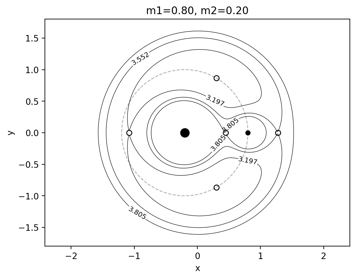
Part (b)
def simulate(sim, Norbits, Noutputs = 1000):
# runs the simulation and makes some plots of the output
times = np.linspace(0, Norbits*2*np.pi, Noutputs)
n = sim.orbits()[0].n
x1 = np.zeros(Noutputs)
y1 = np.zeros(Noutputs)
x2 = np.zeros(Noutputs)
y2 = np.zeros(Noutputs)
x3 = np.zeros(Noutputs)
y3 = np.zeros(Noutputs)
vx3 = np.zeros(Noutputs)
vy3 = np.zeros(Noutputs)
a = np.zeros(Noutputs)
e = np.zeros(Noutputs)
theta = np.zeros(Noutputs)
theta2 = np.zeros(Noutputs)
r1 = np.zeros(Noutputs)
r2 = np.zeros(Noutputs)
for i,t in enumerate(times):
sim.integrate(t, exact_finish_time=1)
x1[i] = sim.particles[0].x
y1[i] = sim.particles[0].y
x2[i] = sim.particles[1].x
y2[i] = sim.particles[1].y
x3[i] = sim.particles[2].x
y3[i] = sim.particles[2].y
vx3[i] = sim.particles[2].vx
vy3[i] = sim.particles[2].vy
a[i] = sim.orbits()[1].a
e[i] = sim.orbits()[1].e
theta2[i] = sim.particles[1].theta
theta[i] = sim.particles[2].theta
r1[i] = np.sqrt((x3[i]-x1[i])**2+(y3[i]-y1[i])**2)
r2[i] = np.sqrt((x3[i]-x2[i])**2+(y3[i]-y2[i])**2)
# compute Jacobi constant (eq. 3.36)
m1 = sim.particles[0].m
m2 = sim.particles[1].m
CJ = 2*(m1/r1 + m2/r2) + 2*n*(x3*vy3-y3*vx3) -vx3**2-vy3**2
# go into the rotating frame
def rotated(x,y,M):
xn = x*np.cos(M) + y*np.sin(M)
yn = -x*np.sin(M) + y*np.cos(M)
return xn, yn
x1, y1 = rotated(x1, y1, theta2)
x2, y2 = rotated(x2, y2, theta2)
x3, y3 = rotated(x3, y3, theta2)
# plots:
# trajectory (Fig 3.16, Fig 3.17)
fig = plt.figure()
#plt.plot(x1, y1)
plt.plot(x2, y2, 'r')
op, = plt.plot(x3, y3, lw=1) # trajectory of test particle
plt.plot(x1[-1], y1[-1], 'ro') # m1 location
plt.plot(x2[-1], y2[-1], 'ro') # m2 location
lim = 1.2
plt.ylim((-lim,lim))
plt.xlim((-lim,lim))
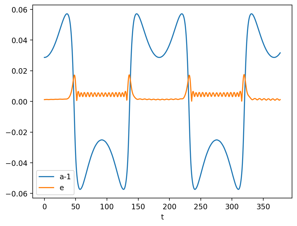
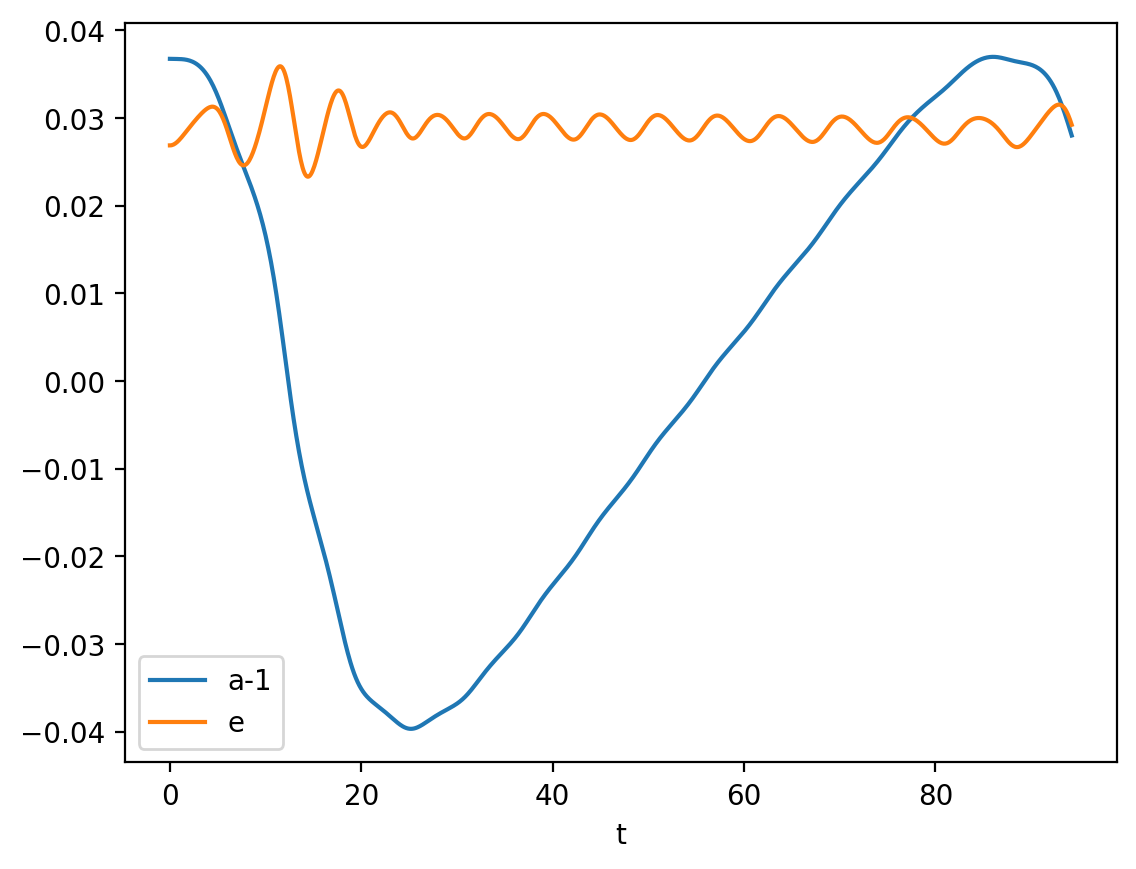
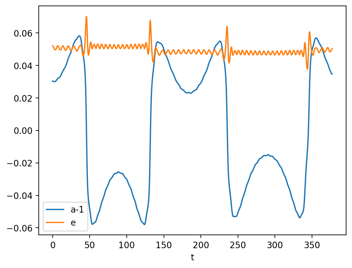
# a and e as function of time (Fig. 3.19)
plt.figure()
plt.plot(times, a-1, label='a-1')
plt.plot(times, e, label='e')
plt.legend()
plt.xlabel('t')
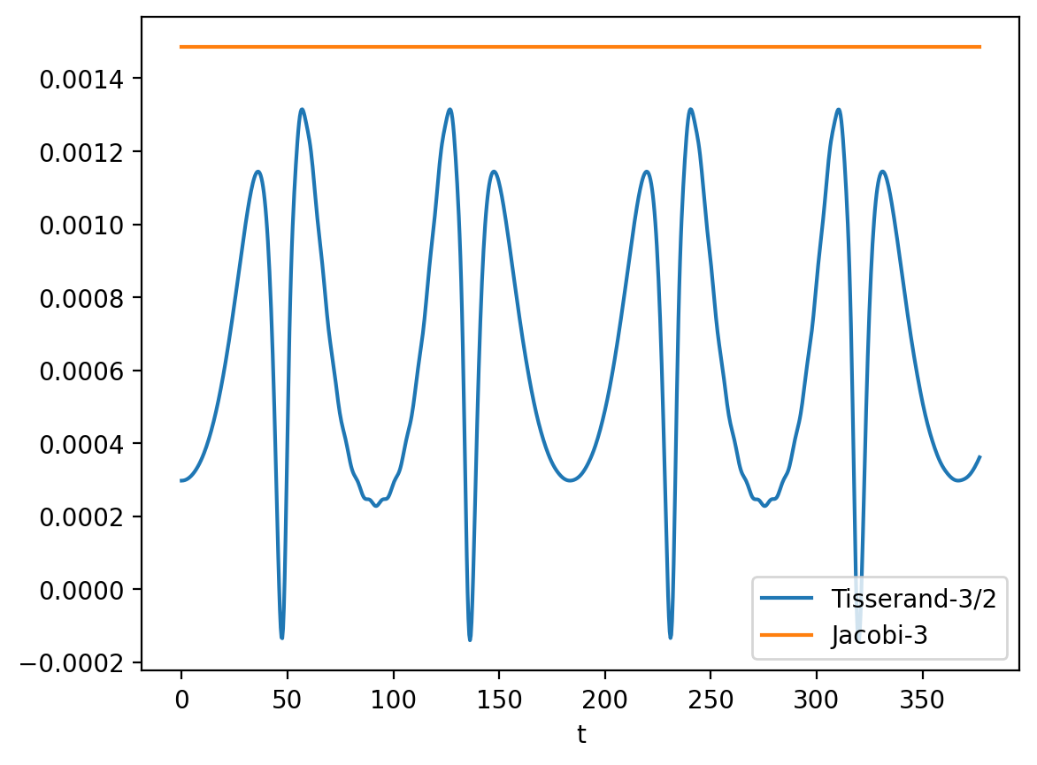
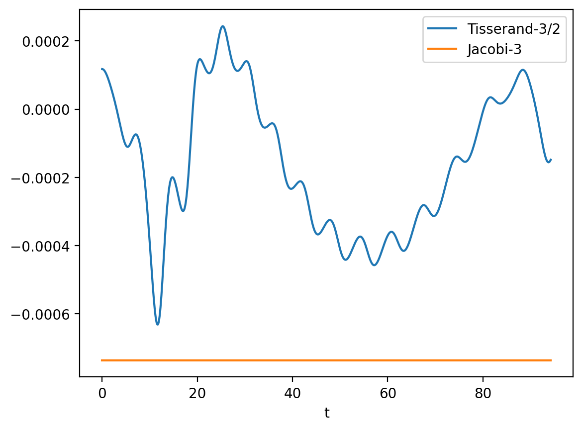
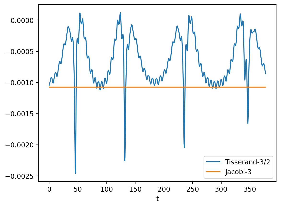
# Jacobi constant/Tisserand approx against time
plt.figure()
CT = 0.5/a + (a*(1-e*e))**0.5 # Tisserand eq. (3.46)
plt.plot(times, CT-1.5, label='Tisserand-3/2')
plt.plot(times, CJ-3, label='Jacobi-3')
plt.legend()
plt.xlabel('t')
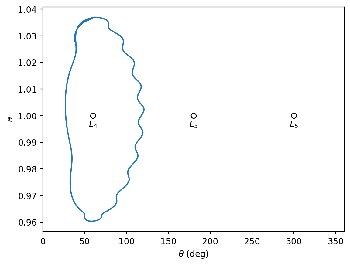
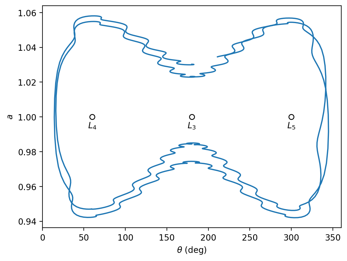
# a vs theta (Fig. 3.18)
plt.figure()
# we can get the angle directly from x3,y3, but I also stored the longitudes as a double-check
#theta = np.degrees(np.mod(np.arctan2(y3,x3),2*np.pi))
plt.plot(np.degrees(np.mod(theta-theta2, 2*np.pi)),a)
plt.plot(60, 1, marker='o', mfc='none', mec='black')
plt.annotate(r"$L_4$", (60,1), xytext=(0,-5), textcoords="offset points", ha="center", va="top")
plt.plot(180, 1, marker='o', mfc='none', mec='black')
plt.annotate(r"$L_3$", (180,1), xytext=(0,-5), textcoords="offset points", ha="center", va="top")
plt.plot(300, 1, marker='o', mfc='none', mec='black')
plt.annotate(r"$L_5$", (300,1), xytext=(0,-5), textcoords="offset points", ha="center", va="top")
plt.xlim((0,360))
plt.xlabel(r'$\theta$ (deg)')
plt.ylabel(r'$a$')
Tadpole from Fig 3.16
plt.close('all')

# Set up circular orbit first
m2 = 0.001
sim = rebound.Simulation()
sim.add(m=1-m2)
sim.add(m=m2, a=1, e=0)
sim.move_to_com()

# check the orbital parameters (should be p_orb=2pi,n=1,a=1,e=0)
p_orb = sim.orbits()[0].P
n = 2*np.pi/p_orb
a = sim.orbits()[0].a
e = sim.orbits()[0].e
print("P,n,a,e = ", p_orb,n,a,e)

# now add the test particle
# tadpole from Fig 3.16
x0, y0 = (0.5, 3**0.5/2)  # L4 location
x,y,xv,vy = (x0 + 0.0065, y0 + 0.0065, 0, 0)
r = (x**2+y**2)**0.5
sim.add(m=0, x=x, y=y, vx=-n*y, vy=n*x)
simulate(sim, 15)
P,n,a,e = 6.283185307179586 1.0 1.0 0.0
First horseshoe example from Fig 3.17
plt.close('all')

# Set up circular orbit first
m2 = 0.000953875
sim = rebound.Simulation()
sim.add(m=1-m2)
sim.add(m=m2, a=1, e=0)
sim.move_to_com()

# horseshoe
# first example from Fig 3.17
x,y,xv,vy = (-0.97668, 0, 0, -0.06118)
#x,y,xv,vy = (-1.02745, 0, 0, 0.04032)
r = (x**2+y**2)**0.5
sim.add(m=0, x=x, y=y, vx=-n*y, vy=n*x + vy)

simulate(sim, 60)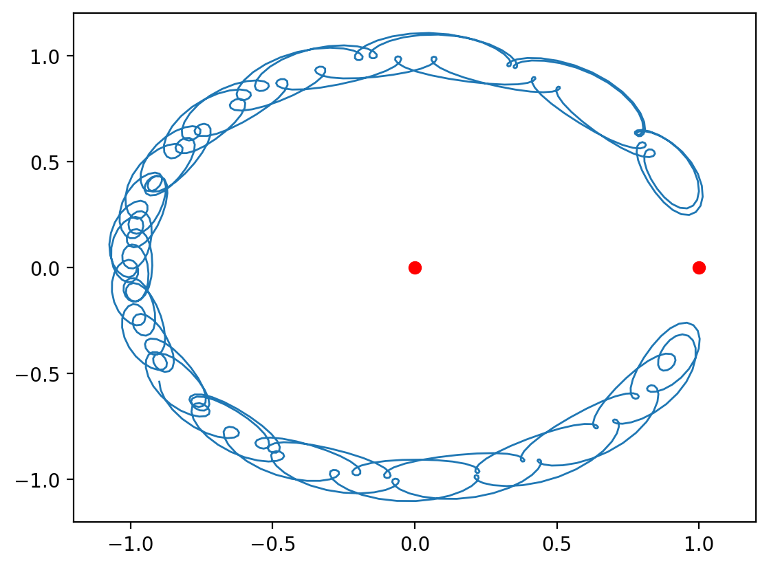
Second horseshoe example from Fig 3.17
plt.close('all')

# Set up circular orbit first
m2 = 0.000953875
sim = rebound.Simulation()
sim.add(m=1-m2)
sim.add(m=m2, a=1, e=0)
sim.move_to_com()

# horseshoe
# second example from Fig 3.17
x,y,xv,vy = (-1.02745, 0, 0, 0.04032)
r = (x**2+y**2)**0.5
sim.add(m=0, x=x, y=y, vx=-n*y, vy=n*x + vy)

simulate(sim, 60)