Week 1 Solutions - PHYS 633 Astrophysical Dynamics

Reading questions¶

(a) For the two-body problem, the constants of motion are the energy and the angular momentum vector (see discussion below eq. 2.28).

(b) The mean motion is the average angular frequency set by the orbital period $T$ , ie. $n=2\pi/T$ (eq. 2.25). For a circular orbit, this is the angular frequency, whereas for an eccentric orbit, the angular frequency changes throughout the orbit but averages to $n$ .

(c) See Fig. 2.5, but it’s good to sketch this yourself and try to label everything (the two foci, semimajor and semiminor axis, peri and apocentre, pericentre distance).

(d) Mean anomaly is $M = n(t-\tau) = 2\pi (t-\tau)/T$ , where time is measured relative to the time of pericentre passage $\tau$ . For an eccentric orbit, this doesn’t have a geometric interpretation but for a circular orbit is just the angle around the orbit.

The true anomaly $f$ is the angle around the orbit as measured from the focus of the orbit. Since the orbiting body moves faster near pericentre than apocentre, the function $f(t)$ is nonlinear in $t$ .

The eccentric anomaly $E$ is the angle as measured from the centre of the circumscribed circle (which has radius equal to the semi-major axis of the ellipse).

(e) Kepler’s equation (2.52) gives the relation between $M$ and $E$ . A given time corresponds to a certain mean anomaly $M$ . Kepler’s equation can then be used to map that to the eccentric anomaly $E$ and then the true anomaly $f$ using equation (2.46) and $r$ using (2.42).

(f) if you want to set up an orbit with semi-major axis a and eccentrity e, how do you choose the initial location and velocity? This is given on p52-53 (section 2.8). The 6D position and velocity map into the six orbital elements $a,e,I,\Omega,\omega$ and $f$ .

(g) This is discussed in section 2.6 p44 on the guiding centre approximation. A spin-synchronized orbiting body always shows the same face to the empty focus of the orbit. So when viewed from the occupied focus, the body appears to rotate slightly over the course of the orbit.

(h) Equation (2.157) for the inclination change can be interpreted as “rate of change of angular momentum is equal to the torque”. For the change of $\Omega$ , you might recognize Equation (2.162) as the equation for precession under an applied torque, where the torque now causes a change of angular momentum that is perpendicular to the current angular momentum vector, causing the angular momentum vector to rotate (precess). Precession velocity = torque / (moment of inertia x sin theta) A diagram helps!

Part 1¶

The goal of Part 1 is to become familiar with how to set up a basic two-body system in REBOUND, and to check that it behaves as expected.

(a) In units with $G=1$ , the orbital frequency is given by $\Omega^2 = (m_1+m_2)/a^3$ and then $P_\mathrm{orb}=2\pi/\Omega$ . Using the value of $a$ from REBOUND (o.a) agrees with the value of o.P (see code below).

(b) Removing the sim.move_to_com() line causes the orbit to slowly drift upwards because the initial velocities are such that the centre of mass has a net velocity given by

(m_1+m_2)v_\mathrm{com} = m_1 v_1 + m_2 v_2

(1)

(eq. 2.106 in section 2.7). In this case, $v_\mathrm{com} = 0.1\times 1.3 / 1.1 = 0.118$ . In one period, the orbit drifts by an amount $0.118\times 18.98\approx 2.24$ in the $y$ -direction.

(c) When you rescale the orbits, the trajectories of the two stars and the relative motion all lie on top of one another, as expected from the discussion in section 2.7 (eq. 2.109). The instantaneous orbit drawn by REBOUND is the orbit of the relative motion. It is offset slightly because it is drawn centred on the primary rather than centred on the origin. (For more on the coordinates used by the code, you can look at this video, or also p441/442 of the book).

(d) We can use the equations in section 2.8 to evaluate the orbital elements if we take $G=1$ . Using $h = x v_y = 1.3$ , $R = 1$ , $V=1.3$ , eq. (2.134) and (2.135) give the same values of $a$ and $e$ as REBOUND (see below).

From eq. (2.135), $e=0$ for $a = h^2/(m_1+m_2)$ . Then using eq. (2.134),

a = {h^2\over m_1+m_2} = \left({2\over R} - {V^2\over m_1+m_2}\right)^{-1}

(2)

and then since the circular orbit has $R=a$ , we can solve for the corresponding velocity which gives

V_\mathrm{circ} = \sqrt{m_1+m_2\over a}

(3)

or $\sqrt{1.1}$ for our values. Checking numerically, this does indeed give a circular orbit in REBOUND. Smaller velocities than this give an eccentric orbit where the initial location is the apastron, whereas larger value give an eccentric orbit where the initial location is the periastron.

%matplotlib widget
import matplotlib.pyplot as plt
import rebound
import time
import numpy as np
plt.close('all')

m1 = 1
m2 = 0.1

# Scaling factors to rescale the orbit (see section 2.7)
scale1 = -(1 + m1/m2)
scale2 = 1 + m2/m1
#scale1 = 1
#scale2 = 1

# set up the simulation
sim = rebound.Simulation()
sim.add(m=m1)
# the initial condition given originally
sim.add(m=m2, x=1, vy=1.3)
# the next line chooses a velocity to give a circular orbit
#sim.add(m=0.1, x=1, vy=1.1**0.5)
sim.move_to_com()

# plot the positions and instantaneous orbit
op = rebound.OrbitPlot(sim, periastron=True)

# output info about the particles and the orbit
for p in sim.particles:
    print(p.x, p.y, p.z)
for o in sim.orbits(): 
    print(o)

# The predicted orbital period is 2pi/Omega where Omega^2 = M/a^3 (since G=1)
print('Orbital period = ', o.P, ' Predicted value = ', 2*np.pi * (o.a**3/1.1)**0.5)

print("v_com = ", 0.1*1.3/1.1)
print("v_circ = ", 1.1**0.5)

-0.09090909090909091 0.0 0.0
0.9090909090909091 0.0 0.0
<rebound.Orbit instance, a=2.1568627450980395 e=0.5363636363636364 inc=0.0 Omega=0.0 omega=0.0 f=0.0>
Orbital period =  18.97655132331586  Predicted value =  18.97655132331586
v_com =  0.11818181818181818
v_circ =  1.0488088481701516

p_orb = sim.orbits()[0].P

# store the positions of the primary and secondary
Noutputs = 100
times = np.linspace(0, 1.0*p_orb, Noutputs)
x1vec = np.zeros(Noutputs)
y1vec = np.zeros(Noutputs)
x2vec = np.zeros(Noutputs)
y2vec = np.zeros(Noutputs)
x1vec[0] = sim.particles[0].x
y1vec[0] = sim.particles[0].y
x2vec[0] = sim.particles[1].x
y2vec[0] = sim.particles[1].y
op2, = plt.plot(scale2 * x2vec[:1], scale2 * y2vec[:1], 'C1')
op3, = plt.plot(scale1 * x1vec[:1], scale1 * y1vec[:1], 'C0')
op4, = plt.plot(x2vec[:1]-x1vec[:1], y2vec[:1]-y1vec[:1], 'C2--')

for i in range(100):
    # integrate for 1% of the orbit
    op.sim.integrate(times[i])

    # store the trajectory of primary and secondary
    x2vec[i] = sim.particles[1].x
    y2vec[i] = sim.particles[1].y
    x1vec[i] = sim.particles[0].x
    y1vec[i] = sim.particles[0].y

    # update the plot to animate it
    op.update() 
    op2.set_data((scale2 * x2vec[:i+1], scale2 * y2vec[:i+1])) 
    op3.set_data((scale1 * x1vec[:i+1], scale1 * y1vec[:i+1])) 
    op4.set_data((x2vec[:i+1]-x1vec[:i+1], y2vec[:i+1]-y1vec[:i+1])) 
    time.sleep(0.001)
    op.fig.canvas.draw()

# predicting the orbital elements for part (d)
h = 1.3
V = 1.3
R = 1
a = 1/((2/R) - V**2/(m1+m2)) # (2.134)
e = (1 - h**2 / (a*(m1+m2)))**0.5
print(a, e)

2.156862745098039 0.5363636363636363

Part 2¶

Guiding Centre¶

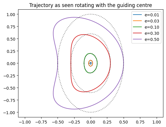
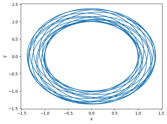
In the guiding centre approximation, an eccentric orbit is decomposed into a reverse elliptical motion around the guiding centre, that itself moves around the centre of mass in a circle with the mean motion $n$ . To test this, we simulate an orbit and then move into the frame rotating with the mean motion.

%matplotlib inline
import matplotlib.pyplot as plt
import rebound
import time
import numpy as np
plt.close('all')

def simulate(e):
    # set up simulation
    sim = rebound.Simulation()
    sim.add(m=1)
    sim.add(m=0, a=1, e=e)
    sim.move_to_com()

    p_orb = sim.orbits()[0].P
    n = 2*np.pi/p_orb
    a = sim.orbits()[0].a
    e = sim.orbits()[0].e
    #print("P,a,e = ", p_orb,a,e)

    # integrate for 1 orbit and store the position of the secondary
    Noutputs = 100
    times = np.linspace(0, 1.0*p_orb, Noutputs)
    x = np.zeros(Noutputs)
    y = np.zeros(Noutputs)
    for i,time in enumerate(times):
        sim.integrate(time, exact_finish_time=1)
        x[i] = sim.particles[1].x
        y[i] = sim.particles[1].y

    # guiding centre location
    M = n * times
    x0 = a * np.cos(M)
    y0 = a * np.sin(M)

    # location relative to guiding centre
    dx = x-x0
    dy = y-y0
    # rotate coordinates
    dx1 = dx*np.cos(M) + dy*np.sin(M)
    dy1 = -dx*np.sin(M) + dy*np.cos(M)

    # plot the motion in this frame and the analytic prediction
    plt.plot(dx1, dy1, label = 'e=%.2f' % (e,))
    plt.plot(-a*e*np.cos(M), 2*a*e*np.sin(M), "k:", alpha=0.6)

    #residual
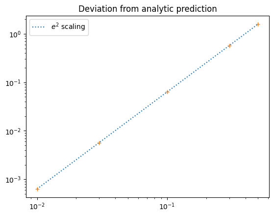
    err2 = np.sum( (dx1+a*e*np.cos(M))**2 + (dy1-2*a*e*np.sin(M))**2)
    #print("e=", e, " rms error / e^2 = ", np.sqrt(err2)/e**2)

    return np.sqrt(err2)


plt.figure()
eccs = (0.01, 0.03, 0.1, 0.3, 0.5)
err = np.zeros(len(eccs))

for i, e in enumerate(eccs):
    err[i] = simulate(e)
    
# plot limits
lim = 2.2 * 0.5
plt.ylim((-lim,lim))
plt.xlim((-lim,lim))
plt.title("Trajectory as seen rotating with the guiding centre")
plt.legend()
plt.show()

plt.figure()
plt.plot((eccs[0],eccs[-1]), (err[0], err[0]*(eccs[-1]/eccs[0])**2), ":", label=r"$e^2$ scaling")
plt.plot(eccs, err, '+')
plt.yscale('log')
plt.xscale('log')
plt.title('Deviation from analytic prediction')
plt.legend()
plt.show()

Applying forces¶

Radial and tangential forces:

%matplotlib inline
import matplotlib.pyplot as plt
import rebound
import time
import numpy as np
plt.close('all')

def do_sim(c, Norbits=10, force='radial'):
    
    sim = rebound.Simulation()
    sim.add(m=1)
    m2 = 1e-6
    sim.add(m=m2, a=1, e=0)
    sim.move_to_com()

    ps = sim.particles
    def starkForce(reb_sim):
        x = ps[1].x
        y = ps[1].y
        r = (x**2+y**2)**0.5
        if force == 'radial':
            # radial force
            ps[1].ax += c * x/r
            ps[1].ay += c * y/r
        elif force == 'tangential':
            # azimuthal force
            ps[1].ax += -c * y/r
            ps[1].ay += c * x/r
    sim.additional_forces = starkForce

    p_orb = sim.orbits()[0].P
    n = 2*np.pi/p_orb
    a = sim.orbits()[0].a
    e = sim.orbits()[0].e
    print("P,a,e = ", p_orb,a,e)

    # store the position of the secondary
    Noutputs = 1000
    times = np.linspace(0, Norbits*p_orb, Noutputs)
    x = np.zeros(Noutputs)
    y = np.zeros(Noutputs)
    a = np.zeros(Noutputs)
    e = np.zeros(Noutputs)
    Omega = np.zeros(Noutputs)
    inc = np.zeros(Noutputs)
    ener = np.zeros(Noutputs)
    h = np.zeros(Noutputs)
    for i,time in enumerate(times):
        sim.integrate(time, exact_finish_time=1)
        x[i] = sim.particles[1].x
        y[i] = sim.particles[1].y
        a[i] = sim.orbits()[0].a
        e[i] = sim.orbits()[0].e
        Omega[i] = sim.orbits()[0].Omega
        inc[i] = sim.orbits()[0].inc
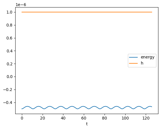
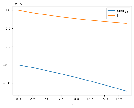
        ener[i] = sim.energy()
        hx,hy,h[i] = sim.angular_momentum()

    plt.figure()
    plt.plot(x,y)
    plt.xlabel('x')
    plt.ylabel('y')

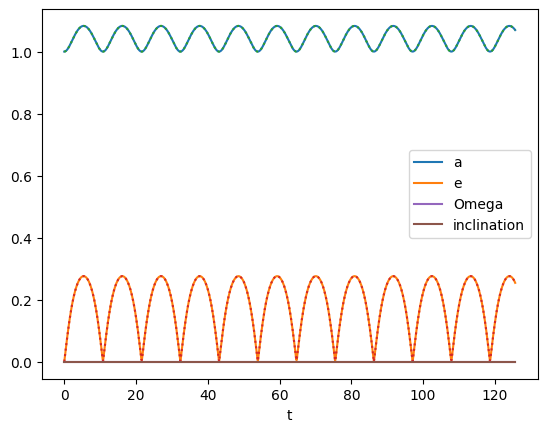
    plt.figure()
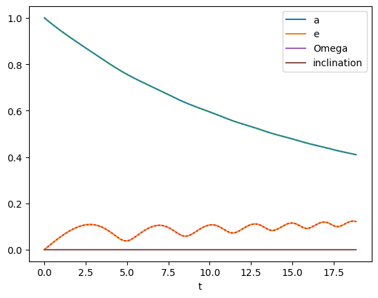
    plt.plot(times, a, label = 'a')
    plt.plot(times, e, label = 'e')
    plt.plot(times, -m2*0.5/ener, ":")   # semi-major axis from the energy
    plt.plot(times, (1 + 2*h*h*ener/m2**3)**0.5, ":")   # eccentricity from h and E
    plt.plot(times, Omega, label = 'Omega')
    plt.plot(times, inc, label = 'inclination')
    plt.legend()
    plt.xlabel('t')

    plt.figure()
    plt.plot(times, ener, label='energy')
    plt.plot(times, h, label='h')
    plt.legend()
    plt.xlabel('t')

# radial force
do_sim(0.1, Norbits=20, force='radial')

P,a,e =  6.283182165589292 1.0000000000000002 2.2204438288064844e-16

# tangential force
do_sim(-0.03, Norbits=3, force='tangential')

P,a,e =  6.283182165589292 1.0000000000000002 2.2204438288064844e-16

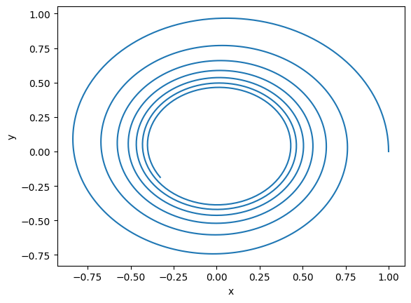
For the normal force, we need to plot in 3D:

%matplotlib widget
import matplotlib.pyplot as plt
from mpl_toolkits.mplot3d import Axes3D  # needed for 3D projection
import rebound
import time
import numpy as np
plt.close('all')

sim = rebound.Simulation()
sim.add(m=1)
m2 = 1e-6
sim.add(m=m2, a=1, e=0.5, inc=np.pi/3, Omega=0.1)
sim.move_to_com()

ps = sim.particles
c = 0.03
def starkForce(reb_sim):
    x = ps[1].x
    y = ps[1].y
    z = ps[1].z
    vx = ps[1].vx
    vy = ps[1].vy
    vz = ps[1].vz
    hx = y*vz-z*vy
    hy = -x*vz+z*vx
    hz = x*vy-y*vx
    h = (hx*hx + hy*hy + hz*hz)**0.5
    # force in direction of instantaneous ang mom vector
    ps[1].ax += c * hx/h
    ps[1].ay += c * hy/h
    ps[1].az += c * hz/h

sim.additional_forces = starkForce

p_orb = sim.orbits()[0].P
n = 2*np.pi/p_orb
a = sim.orbits()[0].a
e = sim.orbits()[0].e
print("P,a,e = ", p_orb,a,e)

# store the position of the secondary
Noutputs = 1000
times = np.linspace(0, 6.5*p_orb, Noutputs)
x = np.zeros(Noutputs)
y = np.zeros(Noutputs)
z = np.zeros(Noutputs)
a = np.zeros(Noutputs)
e = np.zeros(Noutputs)
Omega = np.zeros(Noutputs)
inc = np.zeros(Noutputs)
ener = np.zeros(Noutputs)
h = np.zeros(Noutputs)
for i,time in enumerate(times):
    sim.integrate(time, exact_finish_time=1)
    x[i] = sim.particles[1].x
    y[i] = sim.particles[1].y
    z[i] = sim.particles[1].z
    a[i] = sim.orbits()[0].a
    e[i] = sim.orbits()[0].e
    Omega[i] = sim.orbits()[0].Omega
    inc[i] = sim.orbits()[0].inc
    ener[i] = sim.energy()
    hx,hy,h[i] = sim.angular_momentum()

fig = plt.figure()
ax = fig.add_subplot(111, projection='3d')

ax.plot(x, y, z)

ax.set_xlabel('x')
ax.set_ylabel('y')
ax.set_zlabel('z')

ax.set_xlim(-1, 1)
ax.set_ylim(-1, 1)
ax.set_zlim(-1, 1)

plt.figure()
plt.plot(times, a, label = 'a')
plt.plot(times, e, label = 'e')
plt.plot(times, Omega, label = 'Omega')
plt.plot(times, inc, label = 'inclination')
plt.legend()
plt.xlabel('t')
plt.show()

P,a,e =  6.283182165589295 1.0000000000000007 0.5000000000000003

Velocity space¶

%matplotlib inline
import matplotlib.pyplot as plt
import rebound
import time
import numpy as np
plt.close('all')

def do_sim(e=0):
    sim = rebound.Simulation()
    sim.add(m=1)
    sim.add(m=0, a=1, e=e, omega=0)
    sim.move_to_com()
    
    # store the position and velocity of the secondary
    Noutputs = 1000
    times = np.linspace(0, 1.0*p_orb, Noutputs)
    x = np.zeros(Noutputs)
    y = np.zeros(Noutputs)
    vx = np.zeros(Noutputs)
    vy = np.zeros(Noutputs)
    for i,time in enumerate(times):
        sim.integrate(time, exact_finish_time=1)
        x[i] = sim.particles[1].x
        y[i] = sim.particles[1].y
        vx[i] = sim.particles[1].vx
        vy[i] = sim.particles[1].vy

    # plot the motion in this frame and the analytic prediction
    return x,y,vx,vy

n = 1
a = 1
p_orb = 2*np.pi

plt.figure()
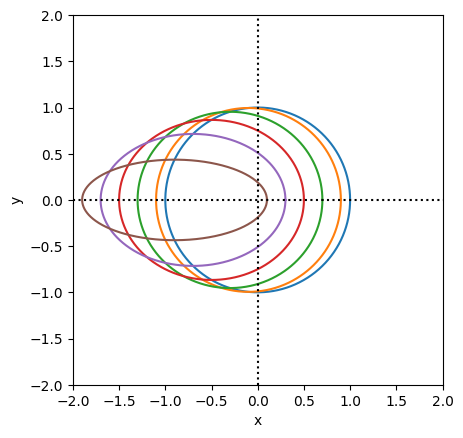
for e in (0, 0.1, 0.3, 0.5, 0.7, 0.9):
    x,y,_,_ = do_sim(e=e)
    plt.plot(x,y, label='e=%.2f' % (e,))

plt.plot([-2,2],[0,0],'k:')
plt.plot([0,0],[-2,2],'k:')
plt.xlabel('x')
plt.ylabel('y')
plt.axis('square')
plt.xlim((-2,2))
plt.ylim((-2,2))

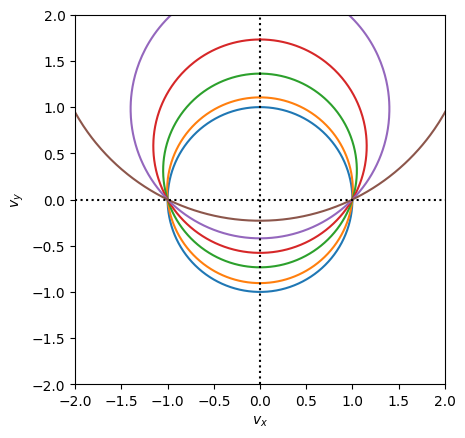
plt.figure()
for e in (0, 0.1, 0.3, 0.5, 0.7, 0.9):
    _,_,vx,vy = do_sim(e=e)
    plt.plot(vx,vy, label='e=%.2f' % (e,))

plt.plot([-2,2],[0,0],'k:')
plt.plot([0,0],[-2,2],'k:')
plt.xlabel(r'$v_x$')
plt.ylabel(r'$v_y$')
plt.axis('square')
plt.xlim((-2,2))
plt.ylim((-2,2))

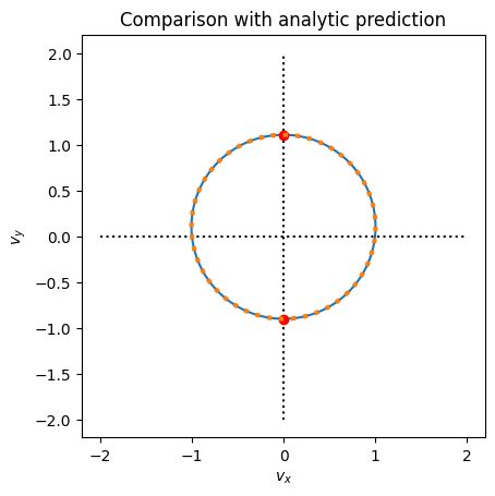
e = 0.1
x,y,vx,vy = do_sim(e=e)

plt.figure()
plt.xlim((-10,10))
plt.ylim((-10,10))
plt.plot([-2,2],[0,0],'k:')
plt.plot([0,0],[-2,2],'k:')
plt.plot(vx, vy)
plt.xlabel(r'$v_x$')
plt.ylabel(r'$v_y$')
plt.axis('square')

# prediction for peri and apo velocities (eqs. 2.35)
vp = n*a*((1+e)/(1-e))**0.5
va = n*a*((1-e)/(1+e))**0.5
plt.plot([0],[vp],'ro')
plt.plot([0],[-va],'ro')

# analytic velocities (eq. 2.36): a circle offset from the origin
f = np.linspace(0,2*np.pi,100)
pref = n*a/(1-e*e)**0.5
vx = pref * np.sin(f)
vy = pref * (e  + np.cos(f))
plt.plot(vx,vy,':',lw=3)

plt.title("Comparison with analytic prediction")


plt.show()